There two problems in this one. Signal Loading and Playing sound


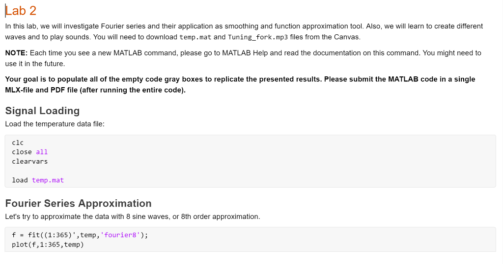
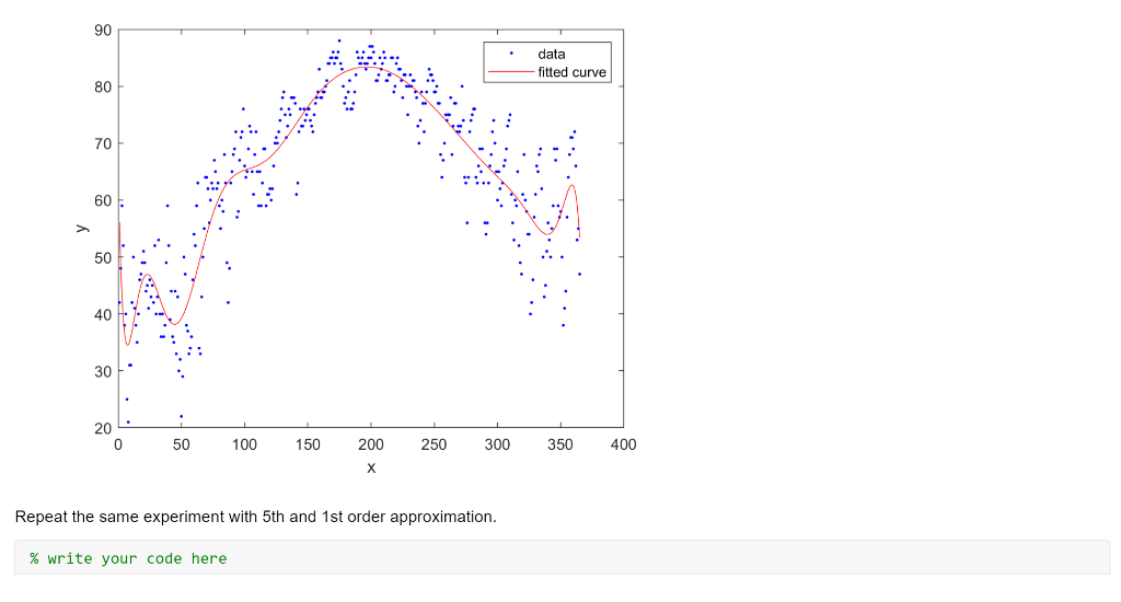
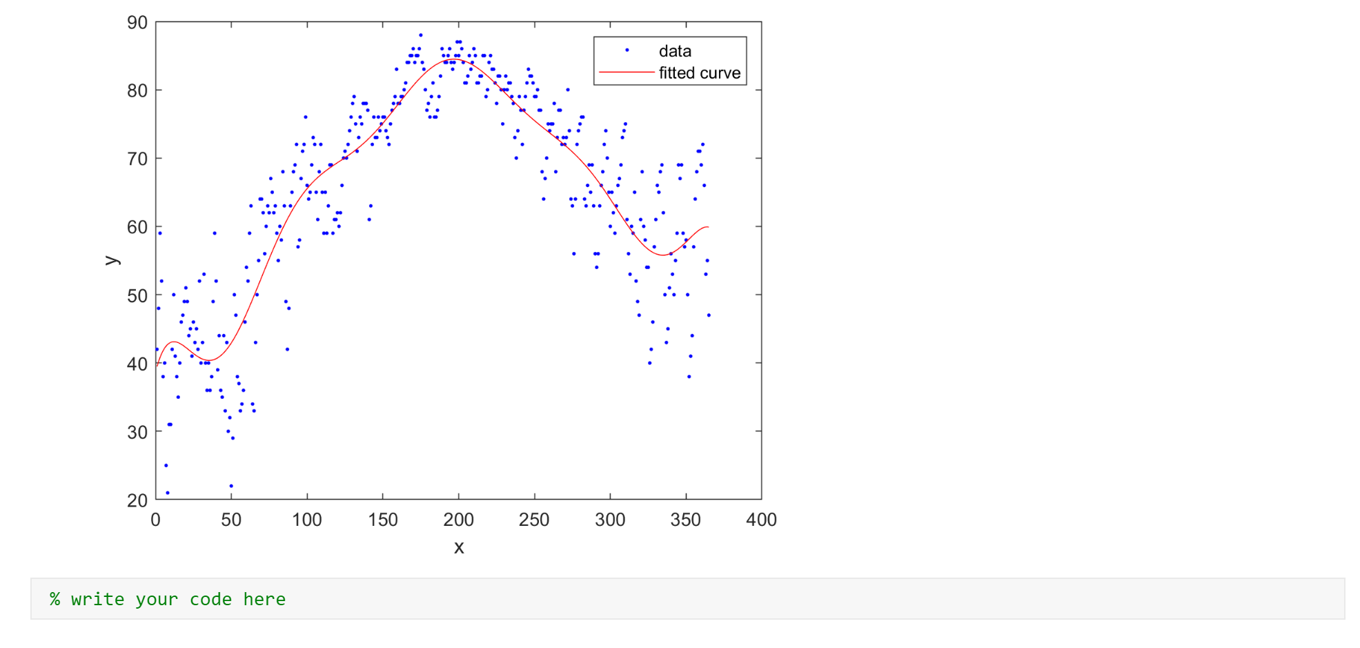
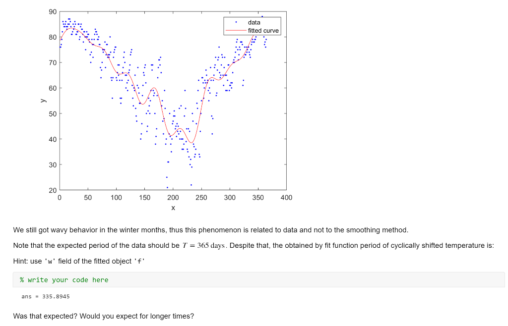
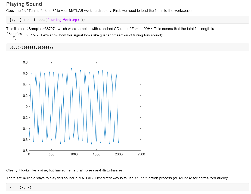
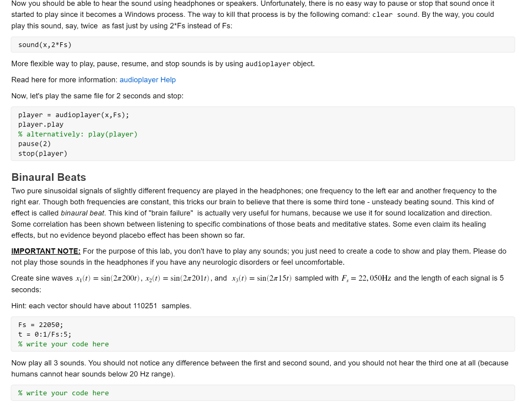
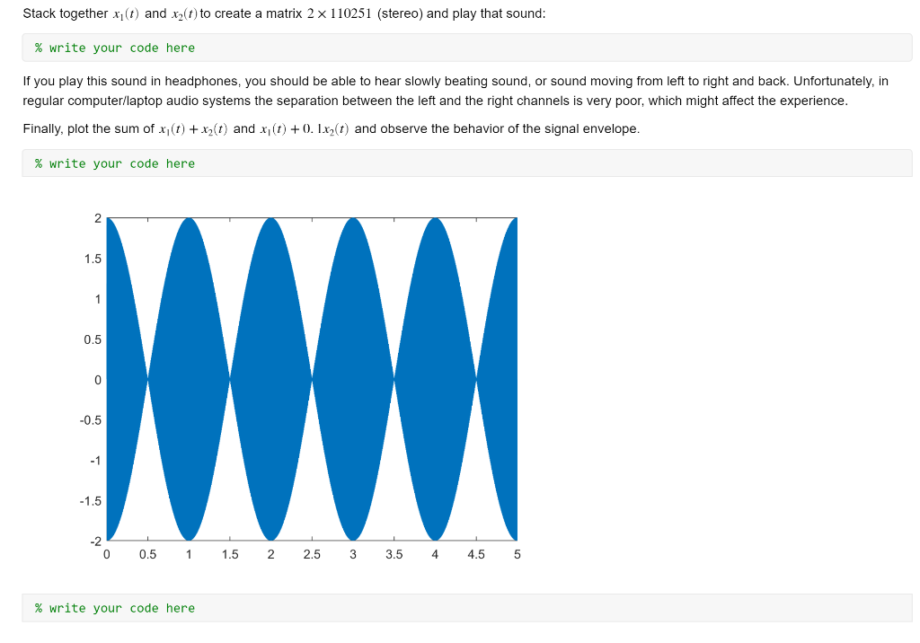
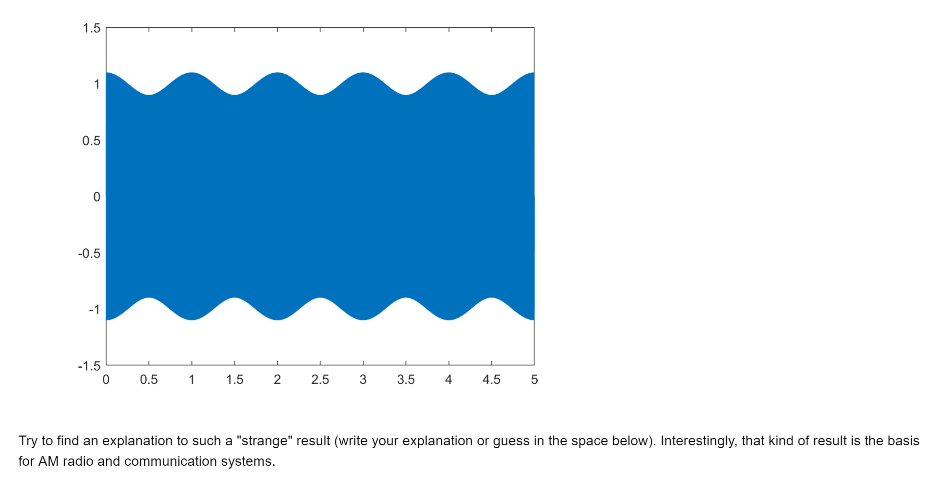
Lab 2 In this lab, we will investigate Fourier series and their application as smoothing and function approximation tool. Also, we will learn to create different waves and to play sounds. You will need to download temp.mat and Tuning_fork.mp3 files from the Canvas. NOTE: Each time you see a new MATLAB command, please go to MATLAB Help and read the documentation on this command. You might need to use it in the future. Your goal is to populate all of the empty code gray boxes to replicate the presented results. Please submit the MATLAB code in a single MLX-file and PDF file (after running the entire code). Signal Loading Load the temperature data file: clc close all clearvars load temp.mat Fourier Series Approximation Let's try to approximate the data with 8 sine waves, or 8th order approximation. f = fit((1:365)', temp,'fourier8'); plot(f, 1:365, temp) 90 data fitted curve 80 70 60 50 40 30 20 0 50 100 150 200 250 300 350 400 X Repeat the same experiment with 5th and 1st order approximation. % write your code here 90 data fitted curve 80 70 60 > . 50 40 30 1 20 0 50 100 150 200 250 300 350 400 x % write your code here 90 data fitted curve 80 70 60 50 40 30 20 0 50 100 150 200 250 300 350 400 As you may see, higher order approximation allows including more details, which might or might not be needed (depends on the application and on the information you'd like to extract). Also, you may note that Fourier series are more "wavy" close to the boundaries of the domain and smoother in the summer months. Is that just coincidence specific for our temperature data, or there is something significant there? That kind of questions we are asking in research. Now, how can we find the answer? If we cyclically shift the entire signal that it will start from the summer and not from January 1st, and still the approximation will be wavy near the ends, then it show that such behavior is typical for Fourier series. Hint: use circshift function to rotate the signal by 182 days. % write your code here 90 data fitted curve 80 70 60 50 40 30 20 0 50 100 150 200 250 300 350 400 We still got wavy behavior in the winter months, thus this phenomenon is related to data and not to the smoothing method. Note that the expected period of the data should be T = 365 days. Despite that, the obtained by fit function period of cyclically shifted temperature is: Hint: use 'w' field of the fitted object 'f' % write your code here ans = 335.8945 Was that expected? Would you expect for longer times? Playing Sound Copy the file "Tuning fork.mp3" to your MATLAB working directory. First, we need to load the file in to the workspace: [x, Fs] = audioread('Tuning fork.mp3'); This file has #Samples=387071 which were sampled with standard CD rate of Fs=44100 Hz. This means that the total file length is #Samples = 8.77scc. Let's show how this signal looks like (just short section of tuning fork sound): F, plot(x(100000:102000)) 0.8 0.6 0.4 0.2 0 -0.2 H -0.4 -0.6 -0.8 0 500 1000 1500 2000 2500 Clearly it looks like a sine, but has some natural noises and disturbances. There are multiple ways to play this sound in MATLAB. First direct way is to use sound function process (or soundsc for normalized audio): sound(x, Fs) Now you should be able to hear the sound using headphones or speakers. Unfortunately, there is no easy way to pause or stop that sound once it started to play since it becomes a Windows process. The way to kill that process is by the following comand: clear sound. By the way, you could play this sound, say, twice as fast just by using 2*Fs instead of Fs: sound(x, 2*Fs) More flexible way to play, pause, resume, and stop sounds is by using audioplayer object. Read here for more information: audioplayer Help Now, let's play the same file for 2 seconds and stop: player = audioplayer(x,Fs); player.play % alternatively: play (player) pause (2) stop(player) Binaural Beats Two pure sinusoidal signals of slightly different frequency are played in the headphones; one frequency to the left ear and another frequency to the right ear. Though both frequencies are constant, this tricks our brain to believe that there is some third tone - unsteady beating sound. This kind of effect is called binaural beat. This kind of "brain failure" is actually very useful for humans, because we use it for sound localization and direction. Some correlation has been shown between listening to specific combinations of those beats and meditative states. Some even claim its healing effects, but no evidence beyond placebo effect has been shown so far. IMPORTANT NOTE: For the purpose of this lab, you don't have to play any sounds; you just need to create a code to show and play them. Please do not play those sounds in the headphones if you have any neurologic disorders or feel uncomfortable. Create sine waves xi(t) = sin(21 200t), xz(t) = sin(212011), and xz(t) = sin(2n 15t) sampled with F, = 22, 050Hz and the length of each signal is 5 seconds: Hint: each vector should have about 110251 samples. FS = 22050; t = 0:1/Fs:5; % write your code here Now play all 3 sounds. You should not notice any difference between the first and second sound, and you should not hear the third one at all (because humans cannot hear sounds below 20 Hz range). % write your code here Stack together xi(t) and x2(t) to create a matrix 2 x 110251 (stereo) and play that sound: % write your code here If you play this sound in headphones, you should be able to hear slowly beating sound, or sound moving from left to right and back. Unfortunately, in regular computer/laptop audio systems the separation between the left and the right channels is very poor, which might affect the experience. Finally, plot the sum of xy(t) + xz(t) and xi(t) +0. Ixz(t) and observe the behavior of the signal envelope. % write your code here 2 1.5 1 0.5 0 -0.5 -1 -1.5 -2 0 0.5 1 1.5 2 2.5 3 3.5 4 4.5 5 % write your code here 1.5 1 0.5 0 -0.5 -1 1 1 -1.5 0 0.5 1 1.5 2. 2.5 3 3.5 4 4.5 5 07 Try to find an explanation to such a "strange" result (write your explanation or guess in the space below). Interestingly, that kind of result is the basis for AM radio and communication systems. Lab 2 In this lab, we will investigate Fourier series and their application as smoothing and function approximation tool. Also, we will learn to create different waves and to play sounds. You will need to download temp.mat and Tuning_fork.mp3 files from the Canvas. NOTE: Each time you see a new MATLAB command, please go to MATLAB Help and read the documentation on this command. You might need to use it in the future. Your goal is to populate all of the empty code gray boxes to replicate the presented results. Please submit the MATLAB code in a single MLX-file and PDF file (after running the entire code). Signal Loading Load the temperature data file: clc close all clearvars load temp.mat Fourier Series Approximation Let's try to approximate the data with 8 sine waves, or 8th order approximation. f = fit((1:365)', temp,'fourier8'); plot(f, 1:365, temp) 90 data fitted curve 80 70 60 50 40 30 20 0 50 100 150 200 250 300 350 400 X Repeat the same experiment with 5th and 1st order approximation. % write your code here 90 data fitted curve 80 70 60 > . 50 40 30 1 20 0 50 100 150 200 250 300 350 400 x % write your code here 90 data fitted curve 80 70 60 50 40 30 20 0 50 100 150 200 250 300 350 400 As you may see, higher order approximation allows including more details, which might or might not be needed (depends on the application and on the information you'd like to extract). Also, you may note that Fourier series are more "wavy" close to the boundaries of the domain and smoother in the summer months. Is that just coincidence specific for our temperature data, or there is something significant there? That kind of questions we are asking in research. Now, how can we find the answer? If we cyclically shift the entire signal that it will start from the summer and not from January 1st, and still the approximation will be wavy near the ends, then it show that such behavior is typical for Fourier series. Hint: use circshift function to rotate the signal by 182 days. % write your code here 90 data fitted curve 80 70 60 50 40 30 20 0 50 100 150 200 250 300 350 400 We still got wavy behavior in the winter months, thus this phenomenon is related to data and not to the smoothing method. Note that the expected period of the data should be T = 365 days. Despite that, the obtained by fit function period of cyclically shifted temperature is: Hint: use 'w' field of the fitted object 'f' % write your code here ans = 335.8945 Was that expected? Would you expect for longer times? Playing Sound Copy the file "Tuning fork.mp3" to your MATLAB working directory. First, we need to load the file in to the workspace: [x, Fs] = audioread('Tuning fork.mp3'); This file has #Samples=387071 which were sampled with standard CD rate of Fs=44100 Hz. This means that the total file length is #Samples = 8.77scc. Let's show how this signal looks like (just short section of tuning fork sound): F, plot(x(100000:102000)) 0.8 0.6 0.4 0.2 0 -0.2 H -0.4 -0.6 -0.8 0 500 1000 1500 2000 2500 Clearly it looks like a sine, but has some natural noises and disturbances. There are multiple ways to play this sound in MATLAB. First direct way is to use sound function process (or soundsc for normalized audio): sound(x, Fs) Now you should be able to hear the sound using headphones or speakers. Unfortunately, there is no easy way to pause or stop that sound once it started to play since it becomes a Windows process. The way to kill that process is by the following comand: clear sound. By the way, you could play this sound, say, twice as fast just by using 2*Fs instead of Fs: sound(x, 2*Fs) More flexible way to play, pause, resume, and stop sounds is by using audioplayer object. Read here for more information: audioplayer Help Now, let's play the same file for 2 seconds and stop: player = audioplayer(x,Fs); player.play % alternatively: play (player) pause (2) stop(player) Binaural Beats Two pure sinusoidal signals of slightly different frequency are played in the headphones; one frequency to the left ear and another frequency to the right ear. Though both frequencies are constant, this tricks our brain to believe that there is some third tone - unsteady beating sound. This kind of effect is called binaural beat. This kind of "brain failure" is actually very useful for humans, because we use it for sound localization and direction. Some correlation has been shown between listening to specific combinations of those beats and meditative states. Some even claim its healing effects, but no evidence beyond placebo effect has been shown so far. IMPORTANT NOTE: For the purpose of this lab, you don't have to play any sounds; you just need to create a code to show and play them. Please do not play those sounds in the headphones if you have any neurologic disorders or feel uncomfortable. Create sine waves xi(t) = sin(21 200t), xz(t) = sin(212011), and xz(t) = sin(2n 15t) sampled with F, = 22, 050Hz and the length of each signal is 5 seconds: Hint: each vector should have about 110251 samples. FS = 22050; t = 0:1/Fs:5; % write your code here Now play all 3 sounds. You should not notice any difference between the first and second sound, and you should not hear the third one at all (because humans cannot hear sounds below 20 Hz range). % write your code here Stack together xi(t) and x2(t) to create a matrix 2 x 110251 (stereo) and play that sound: % write your code here If you play this sound in headphones, you should be able to hear slowly beating sound, or sound moving from left to right and back. Unfortunately, in regular computer/laptop audio systems the separation between the left and the right channels is very poor, which might affect the experience. Finally, plot the sum of xy(t) + xz(t) and xi(t) +0. Ixz(t) and observe the behavior of the signal envelope. % write your code here 2 1.5 1 0.5 0 -0.5 -1 -1.5 -2 0 0.5 1 1.5 2 2.5 3 3.5 4 4.5 5 % write your code here 1.5 1 0.5 0 -0.5 -1 1 1 -1.5 0 0.5 1 1.5 2. 2.5 3 3.5 4 4.5 5 07 Try to find an explanation to such a "strange" result (write your explanation or guess in the space below). Interestingly, that kind of result is the basis for AM radio and communication systems
