This is a MATLAB question based on Computational Methods and Applications. Please show clear code with clear explanation. Thanks. Will up vote.

Down below is the given HW7p1.m

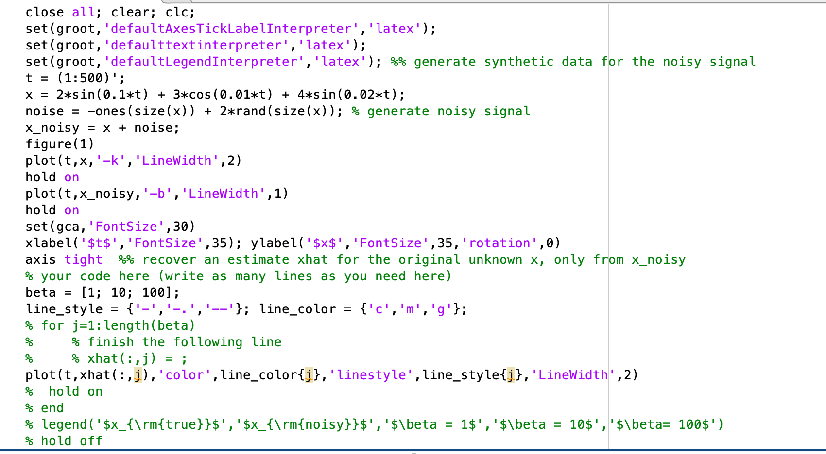
Same code :

-----------------------------------------------

close all; clear; clc;

set(groot,'defaultAxesTickLabelInterpreter','latex');

set(groot,'defaulttextinterpreter','latex');

set(groot,'defaultLegendInterpreter','latex');

%% generate synthetic data for the noisy signal

t = (1:500)';

x = 2*sin(0.1*t) + 3*cos(0.01*t) + 4*sin(0.02*t);

noise = -ones(size(x)) + 2*rand(size(x));

% generate noisy signal

x_noisy = x + noise;

figure(1)

plot(t,x,'-k','LineWidth',2)

hold on

plot(t,x_noisy,'-b','LineWidth',1)

hold on

set(gca,'FontSize',30)

xlabel('$t$','FontSize',35); ylabel('$x$','FontSize',35,'rotation',0)

axis tight

%% recover an estimate xhat for the original unknown x, only from x_noisy

% your code here (write as many lines as you need here)

beta = [1; 10; 100];

line_style = {'-','-.','--'}; line_color = {'c','m','g'};

% for j=1:length(beta)

%

% % finish the following line

% % xhat(:,j) = ;

%

%

plot(t,xhat(:,j),'color',line_color{j},'linestyle',line_style{j},'LineWidth',2)

% hold on

% end

% legend('$x_{ m{true}}$','$x_{ m{noisy}}$','$\beta = 1$','$\beta = 10$','$\beta = 100$')

% hold off

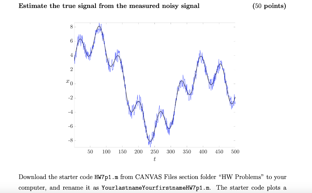
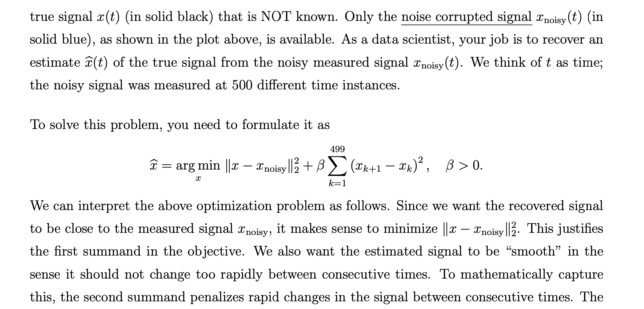
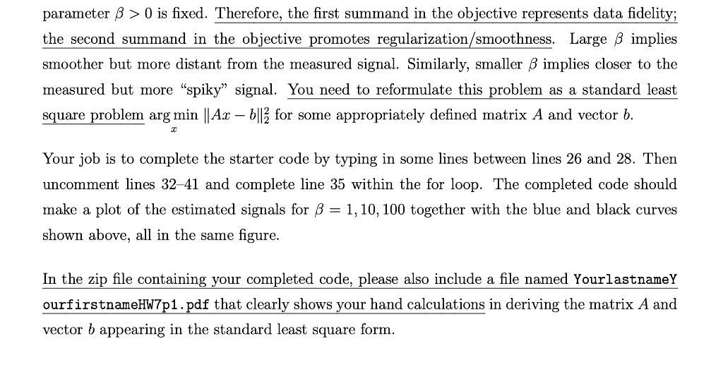
Estimate the true signal from the measured noisy signal (50 points) 8 6 4 2 TO -2 -4 -6 -8 50 100 150 200 300 350 400 450 500 250 t Download the starter code Hw7p1.m from CANVAS Files section folder HW Problems to your computer, and rename it as Yourlastname YourfirstnameHW7p1.m. The starter code plots a true signal x(t) (in solid black) that is NOT known. Only the noise corrupted signal X noisy(t) (in solid blue), as shown in the plot above, is available. As a data scientist, your job is to recover an estimate a(t) of the true signal from the noisy measured signal X noisy(t). We think of t as time; the noisy signal was measured at 500 different time instances. To solve this problem, you need to formulate it as 499 = arg min || 2 Xnoisy ll2 + B (Xk+1 xk)?, B > 0. k=1 We can interpret the above optimization problem as follows. Since we want the recovered signal to be close to the measured signal 0 is fixed. Therefore, the first summand in the objective represents data fidelity; the second summand in the objective promotes regularization/smoothness. Large B implies smoother but more distant from the measured signal. Similarly, smaller B implies closer to the measured but more spiky" signal. You need to reformulate this problem as a standard least square problem arg min ||Ax 6||* for some appropriately defined matrix A and vector b. Your job is to complete the starter code by typing in some lines between lines 26 and 28. Then uncomment lines 32-41 and complete line 35 within the for loop. The completed code should make a plot of the estimated signals for B = 1, 10, 100 together with the blue and black curves shown above, all in the same figure. In the zip file containing your completed code, please also include a file named Yourlastname Y ourfirstnameHW7p1.pdf that clearly shows your hand calculations in deriving the matrix A and vector b appearing in the standard least square form. X = close all; clear; clc; set(groot, 'defaultAxesTickLabelInterpreter', 'latex'); set(groot, 'defaulttextinterpreter', 'latex'); set(groot, 'defaultLegend Interpreter', 'latex'); %% generate synthetic data for the noisy signal t = (1:500)'; 2*sin(0.1*t) + 3*cos(0.01*t) + 4*sin(0.02*t); noise = -ones (size(x)) + 2*rand (size(x)); % generate noisy signal X_noisy = x + noise; figure(1) plot(t,x,'-k', 'LineWidth',2) hold on plot(t,x_noisy,'-b', 'LineWidth',1) hold on set(gca, 'FontSize',30) xlabel('$t$', 'FontSize',35); ylabel('$X$', 'FontSize',35, 'rotation',0) axis tight %% recover an estimate xhat for the original unknown x, only from x_noisy % your code here (write as many lines as you need here) beta [1; 10; 100); line_style {'-','-,','--'}; line_color {'c','m','g'}; % for j=1: length(beta) % finish the following line % xhat(:,j) = ; plot(t, xhat(:,j),'color', line_color{j}, 'linestyle', line_style{j}, 'LineWidth',2) hold on % end % legend ( '$x_{ m{true}}$', '$x_{ m{noisy}}$', '$\beta 1$', '$\beta 10$', '$\beta= 100$') % hold off