This is International Business and Trade subject. Please help me answer the following (briefly and concisely):

1. Differentiate Vertical and Horizontal Foreign Direct Exchange Decisions.

2. What do you think is the significance of Intra- Industry Trade? Explain.

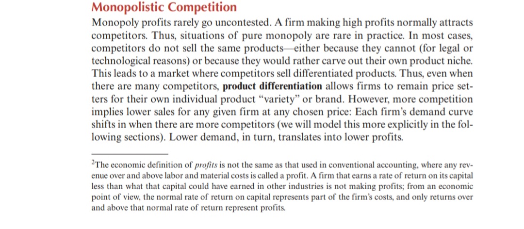
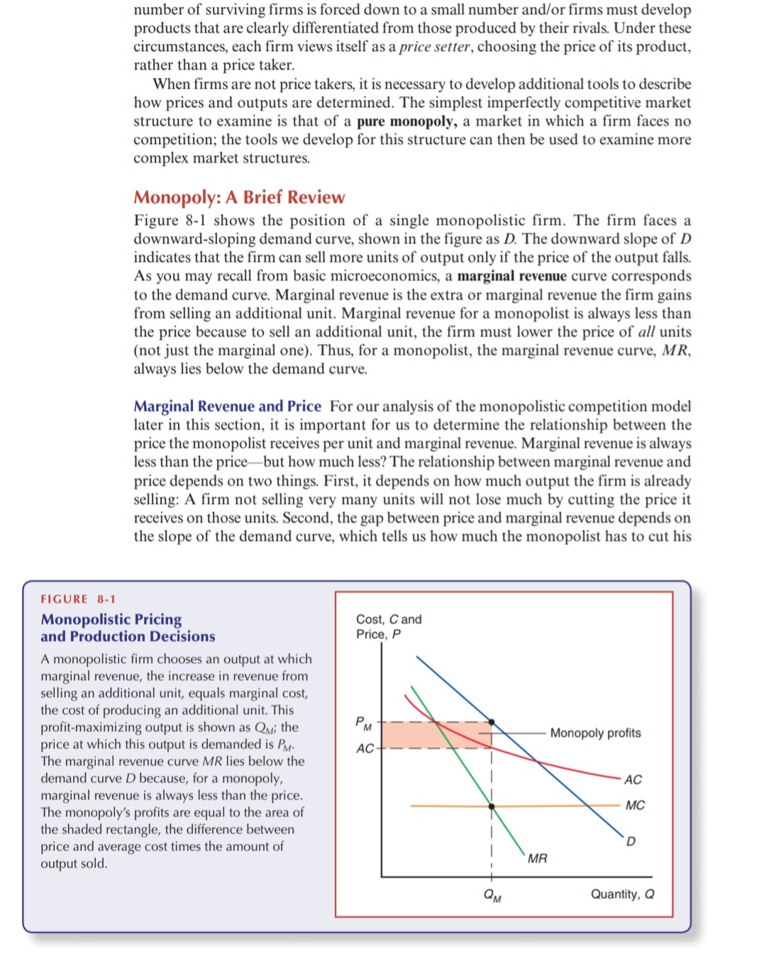
3. Discuss the theory of Imperfect competition and explain the differences between Monopolistic and Oligopolistic competition.

4. What is the relationship between External Economies and International Trade?

5. What is the theory of External Economies?

6. Explain the concept of Economies of Scale.

Notes:

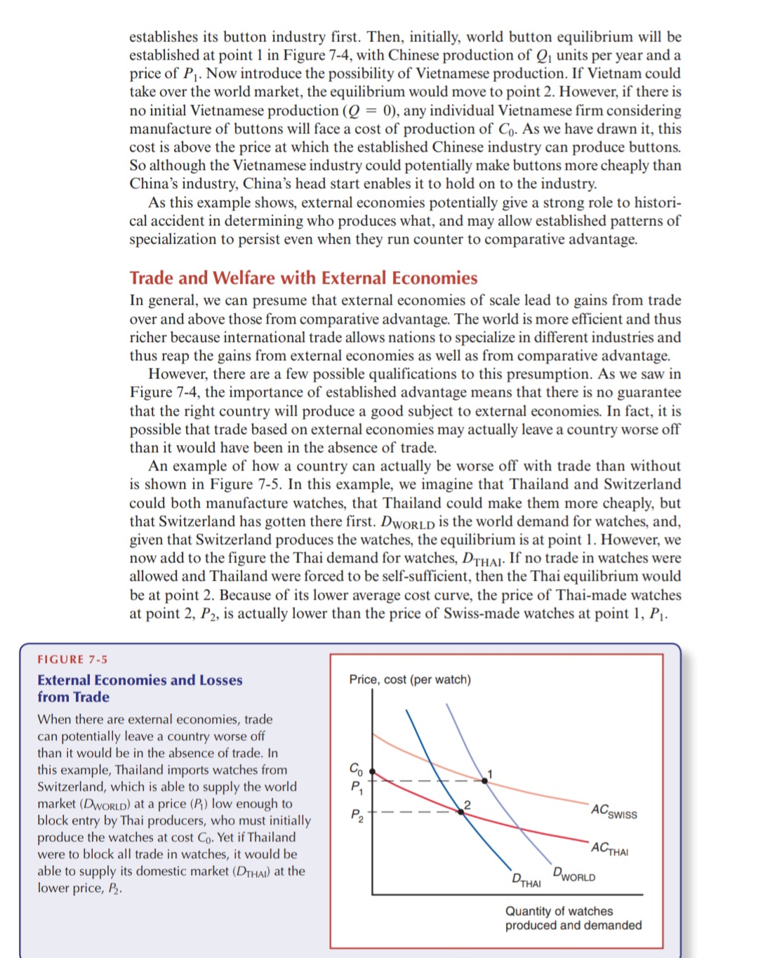
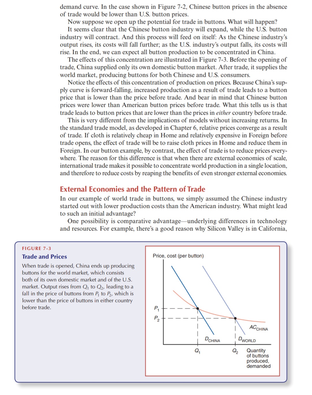
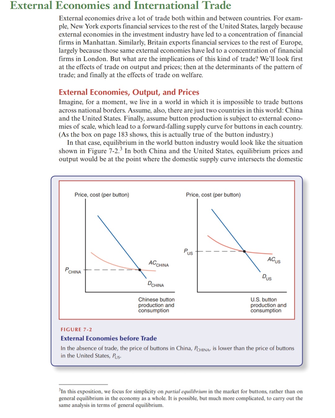
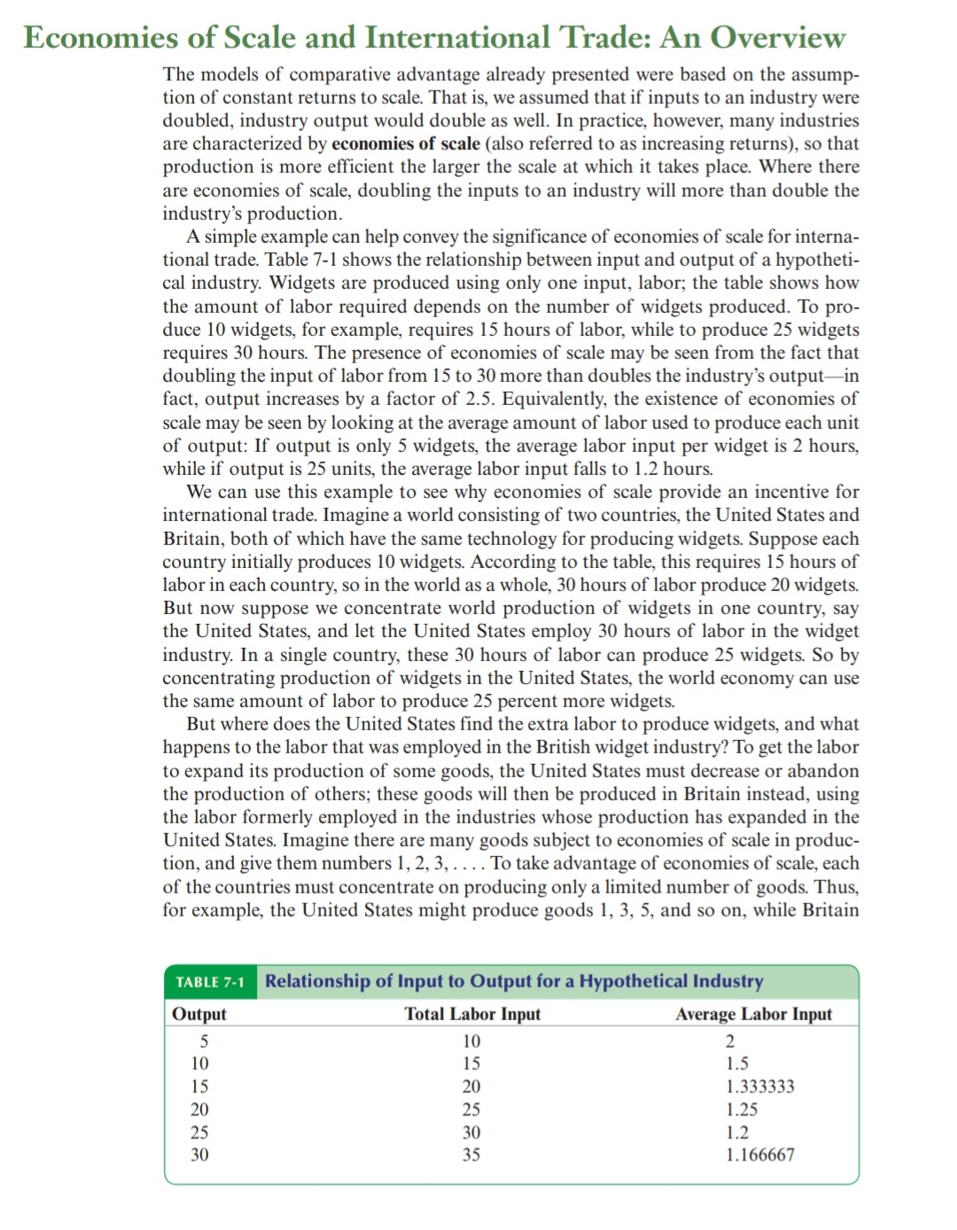
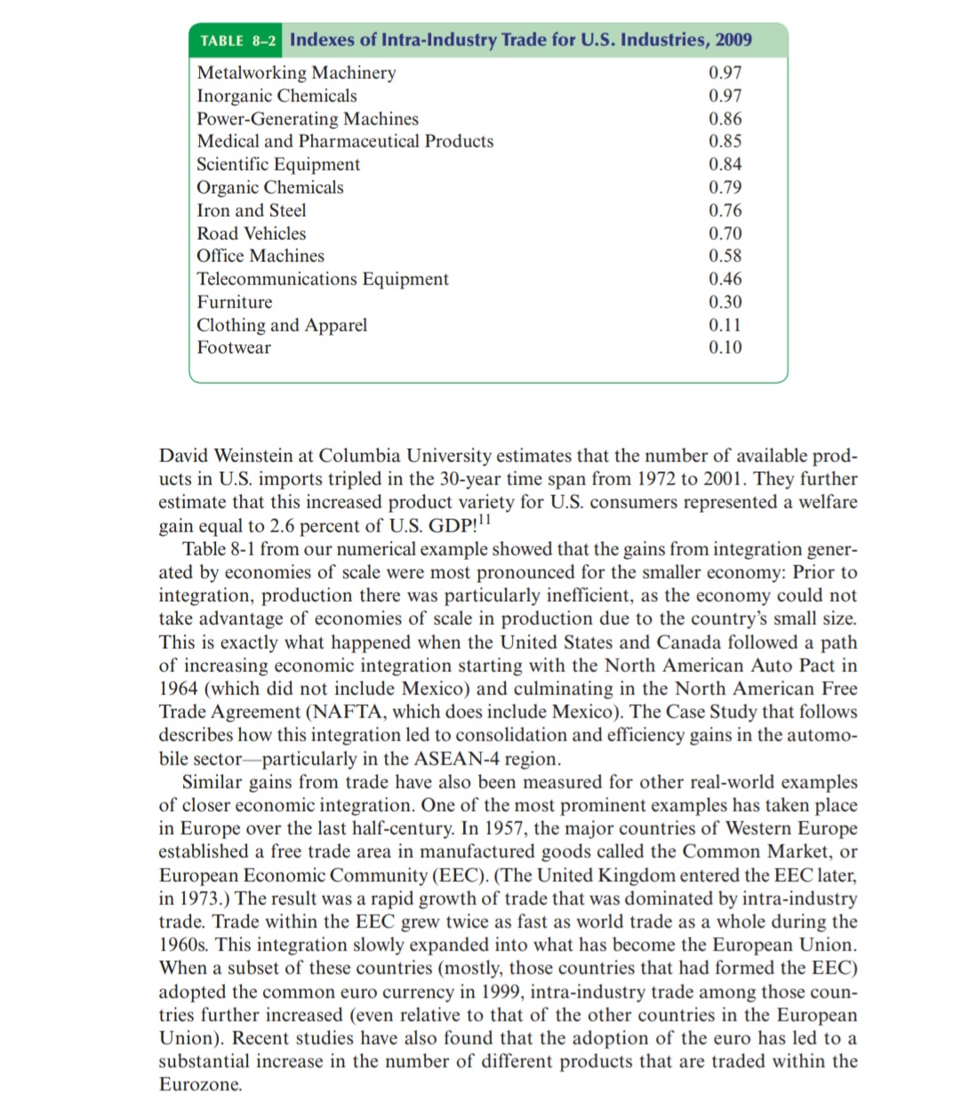
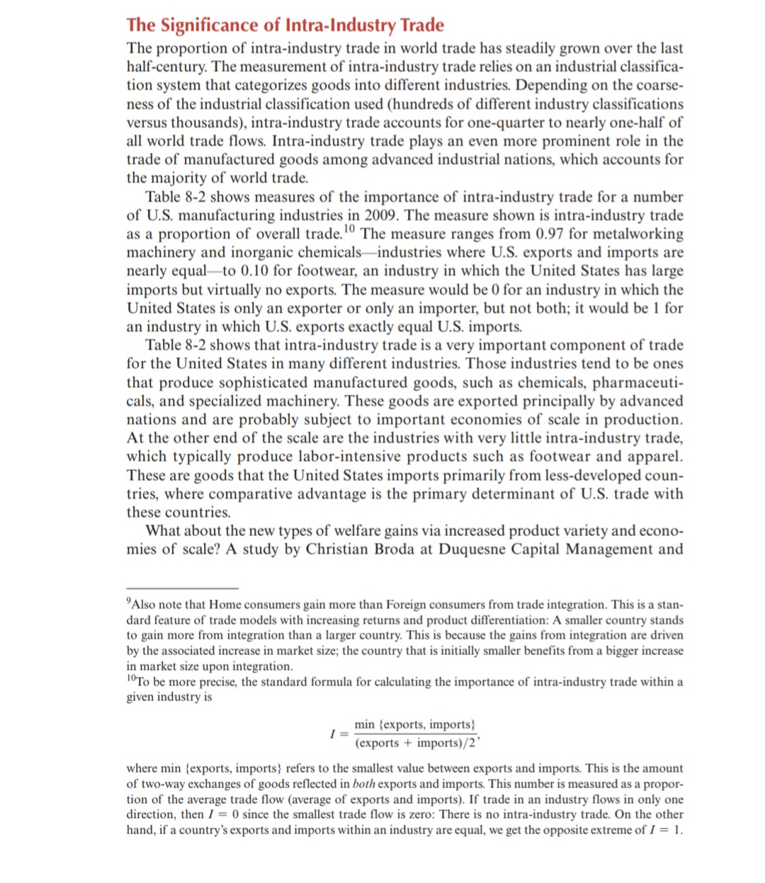
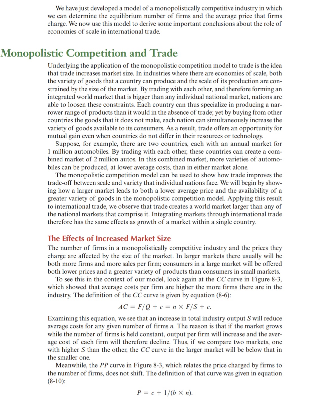
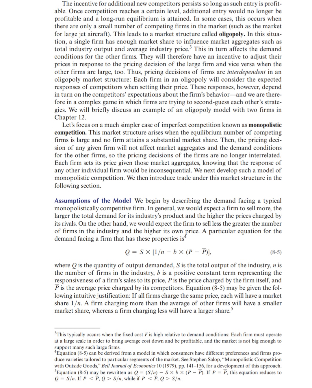
Q units to foreign customers. The most cost-effective way to do this is to build an affili ate in Foreign and become a multinational. Some firms with intermediate cost levels will still want to serve customers in Foreign, but their intended sales Q are low enough that exports, rather than FDI, will be the most cost-effective way to reach those customers. The Vertical FDI Decision A firm's decision to break up its production chain and move parts of that chain to a foreign affiliate will also involve a trade-off between per-unit and fixed costs-so the scale of the firm's activity will again be a crucial element deter- mining this outcome. When it comes to vertical FDI, the key cost saving is not related to the shipment of goods across borders; rather, it involves production cost differences for the parts of the production chain that are being moved. As we previously discussed, those cost differences stem mostly from comparative advantage forces. We will not discuss those cost differences further here, but rather ask why-given those cost differences-all firms do not choose to operate affiliates in low-wage coun- tries to perform the activities that are most labor-intensive and can be performed in a different location. The reason is that, as with the case of horizontal FDI, vertical FDI requires a substantial fixed cost investment in a foreign affiliate in a country with the appropriate characteristics. Again, as with the case of horizontal FDI, there will be a scale cutoff for vertical FDI that depends on the production cost differentials on one hand, and the fixed cost of operating a foreign affiliate on the other hand. Only those firms operating at a scale above that cutoff will choose to perform vertical FDI.establishes its button industry first. Then, initially, world button equilibrium will be established at point 1 in Figure 7-4, with Chinese production of Q. units per year and a price of P]. Now introduce the possibility of Vietnamese production. If Vietnam could take over the world market, the equilibrium would move to point 2. However, if there is no initial Vietnamese production (Q = 0), any individual Vietnamese rm considering manufacture of buttons will face a cost of production of Co. As we have drawn it, this cost is above the price at which the established Chinese industry can produce buttons. So although the Vietnamese industry could potentially make buttons more cheaply than China's industry, China's head start enables it to hold on to the industry. As this example shows, external economies potentially give a strong role to histori- cal accident in determining who produces what, and may allow established patterns of specialization to persist even when they run counter to comparative advantage. Trade and Welfare with External Economies In general, we can presume that external economies of scale lead to gains from trade over and above those from comparative advantage. The world is more efficient and thus richer because international trade allows nations to specialize in different industries and thus reap the gains from external economies as well as from comparative advantage. However, there are a few possible qualifications to this presumption. As we saw in Figure 7-4, the importance of established advantage means that there is no guarantee that the right country will produce a good subject to external economies. In fact, it is possible that trade based on external economies may actually leave a country worse off than it would have been in the absence of trade. An example of how a country can actually be worse off with trade than without is shown in Figure ?-5. In this example, we imagine that Thailand and Switzerland could both manufacture watches, that Thailand could make them more cheaply, but that Switzerland has gotten there first. DWORLD is the world demand for watches, and, given that Switzerland produces the watches, the equilibrium is at point 1. However, we now add to the gure the Thai demand for watches, DTHM. If no trade in watches were allowed and Thailand were forced to be self-sufficient, then the Thai equilibrium would be at point 2. Because of its lower average cost curve, the price of Thai-made watches at point 2, P2, is actually lower than the price of Swiss-made watches at point 1, Pl. FIGURE 7-5 External Economies and losses Price. 0051 (per watch) from Trade When there are external economies, trade can potentially leave a country worse off than It would be in the absence of trade. In this example, Thailand imports watches from Switzerland, which is able to supply the world market (Di-roam) at a price (H) low enough to block entry by Thai producers, who must initially produce the watches at cost Cg. Yet ifThailand were to block all trade in watches, it would be able to supply its domestic market (Drum) at the lower price, Pg. Quantity of watches produced and demanded rather than in Mexico. High-technology industries require a highly skilled work force, and such a work force is much easier to nd in the United States, where 40 percent of the working-age population is college-educated, than in Mexico, where the number is below 16 percent. Similarly, there's a good reason why world button production is concentrated in China, rather than in Germany. Button production is a labor-intensive industry, which is best conducted in a country where the average manufacturing worker earns less than a dollar an hour rather than in a country where hourly compensation is among the highest in the world. However, in industries characterized by external economies of scale, comparative advantage usually provides only a partial explanation of the pattern of trade It was prob- ably inevitable that most of the world's buttons would be made in a relatively low-wage country, but it's not clear that this country necessarily had to be China, and it certainly wasn't necessary that production be concentrated in any particular location within China. So what does determine the pattern of specialization and trade in industries with external economies of scale? The answer, often, is historical contingency: Something gives a particular location an initial advantage in a particular industry, and this advan- tage gets \"locked in\" by external economies of scale even after the circumstances that created the initial advantage are no longer relevant. The financial centers in London and New York are clear examples London became Europe's dominant financial center in the 19th century, when Britain was the world's leading economy and the center of a world-spanning empire It has retained that role even though the empire is long gone and modern Britain is only a middle-sized economic power. New York became America's nancial center thanks to the Erie Canal, which made it the nation's leading port. It has retained that role even though the canal currently is used mainly by recreational boats Often sheer accident plays a key role in creating an industrial concentration. Geog- raphers like to tell the tale of how a tufted bedspread. crafted as a wedding gift by a 19th-century teenager. gave rise to the cluster of carpet manufacturers around Dalton, Georgia. Silicon Valley's existence may owe a lot to the fact that a couple of Stanford graduates named Hewlett and Packard decided to start a business in a garage in that area. Bangalore might not be what it is today if vagaries of local politics had not led Texas Instruments to choose back in 1984, to locate an investment project there rather than in another Indian city. One consequence of the role of history in determining industrial location is that industries aren't always located in the \"right" place: Once a country has established an advantage in an industry. it may retain that advantage even if some other country could potentially produce the goods more cheaply. Figure 7-4, which shows the cost of producing buttons as a function of the number of buttons produced annually, illustrates this point. Two countries are shown: China and Vietnam. The Chinese cost of producing a button is shown as A Comm, the Viet- namese cost as ACVIETNAM. DWORLD represents the world demand for buttons, which we assume can be satised either by China or by Vietnam. Suppose the economies of scale in button production are entirely external to firms. Since there are no economies of scale at the level of the rm. the button industry in each country consists of many small, perfectly competitive rms. Competition there- fore drives the price of buttons down to its average cost. We assume the Vietnamese cost curve lies below the Chinese curve because, say. Vietnamese wages are lower than Chinese wages This means that at any given level of production, Vietnam could manufacture buttons more cheaply than China. One might hope that this would always imply that Vietnam will in fact supply the world market. Unfortunately. this need not be the case. Suppose China. for historical reasons, FIGURE 7-3 demand curve. In the case shown in Figure "3-2, Chinese button prices in the absence of trade would be lower than U. S. button prices. Now suppose we open up the potential for trade in buttons. What will happen? It seems clear that the Chinese button industry will expand, while the US. button industry will contract. And this process will feed on itself: As the Chinese industry's output rises, its costs will fall further; as the U.S. industry's output falls, its costs will rise. In the end, we can expect all button production to be concentrated in China. The effects of this concentration are illustrated in Figure "if-3. Before the opening of trade, China supplied only its own domestic button market. After trade, it supplies the world market. producing buttons for both Chinese and U. S. consumers. Notice the effects of this concentration of production on prices. Because China's sup- ply curve is forward-falling, increased production as a result of trade leads to a button price that is lower than the price before trade. And bear in mind that Chinese button prices were lower than American button prices before trade. What this tells us is that trade leads to button prices that are lower than the prices in either country before trade. This is very different from the implications of models without increasing returns. In the standard trade model, as developed in Chapter 6, relative prices converge as a result of trade. If cloth is relatively cheap in Home and relativer expensive in Foreign before trade opens, the effect of trade will be to raise cloth prices in Home and reduce them in Foreign. In our but ton example, by contrast, the effect of trade is to reduce prices every- where. The reason for this difference is that when there are external economies of scale, international trade makes it possible to concentrate world production in a single location, and therefore to reduce costs by reaping the benefits of even stronger external economies. External Economies and the Pattern of Trade In our example of world trade in buttons, we simply assumed the Chinese industry started out with lower production costs than the American industry. What might lead to such an initial advantage? One possibility is comparative advantageunderlying differences in technology and resources. For example, there's a good reason why Silicon Valley is in California, Trade and Prices Price. cost {per button} When trade is opened, China ends up producing buttons for the world market, which consists both of its own domestic market and of the U.S. market. Output rises from Q to (2;, leading to a fall in the price of buttons from P1 to P2, which is lower than the price of buttons in either country before trade. External Economies and International Trade External economies drive a lot of trade both within and between countries For exam- ple, New York exports f'mancial services to the rest of the United States, largely because external economies in the investment industry have led to a concentration of nancial rms in Manhattan. Similarly, Britain exports nancial services to the rest of Europe, largely because those same external economies have led to a concentration of nancial rms in London. But what are the implications of this kind of trade? We'll look rst at the effects of trade on output and prices; then at the determinants of the pattern of trade; and nally at the effects of trade on welfare. External Economies, Output, and Prices Imagine, for a moment, we live in a world in which it is impossible to trade buttons across national borders. Assume, also, there are just two countries in this world: China and the United States. Finally, assume button production is subject to external econo- mies of scale, which lead to a forward-falling supply curve for buttons in each country. (As the box on page 183 shows, this is actually true of the button industry.) In that case, equilibrium in the world button industry would look like the situation shown in Figure 7-2.3 In both China and the United States, equilibrium prices and output would be at the point where the domestic supply curve intersects the domestic Price. cost (per button) Price. cost (per button) Chinese button U.S. button production and production and consumption consumption F I G U I! E 7- 2 External Economies before Trade In the absence of trade, the price of buttons in China, P0...\" is lower than the price of buttons in the United States, Js. 3In this exposition. we focus for simplicity on partial equilibrium in the market for buttons. rather than on general equilibrium in the economy as a whole. It is possible. but much more complicated, to carry out the same analysis in terms of general equilibrium. perfectly competitive. Internal economies of scale, by contrast, give large rms a cost advantage over small rms and lead to an imperfectly competitive market structure. Both external and internal economies of scale are important causes of international trade. Because they have different implications for market structure, however, it is dif- cult to discuss both types of scale economybased trade in the same model. We will therefore deal with them one at a time. In this chapter, we focus on external economies; in Chapter 8, on internal economies. The Theory of External Economies As we have already pointed out, not all scale economies apply at the level of the indi- vidual rm. For a variety of reasons, it is often the case that concentrating production of an industry in one or a few locations reduces the industry's costs even if the indi- vidual rms in the industry remain small. When economies of scale apply at the level of the industry rather than at the level of the individual rm, they are called external economies. The analysis of external economies goes back more than a century to the British economist Alfred Marshall, who was struck by the phenomenon of \"industrial districts\"geographical concentrations of industry that could not be easily explained by natural resources. In Marshall's time, the most famous examples included such concentrations of industry as the cluster of cutlery manufacturers in Shefeld and the cluster of hosiery firms in Northampton. There are many modern examples of industries where there seem to be powerful exter- nal economies. In the United States, these examples include the semiconductor industry, concentrated in California's famous Silicon Valley; the investment banking industry, con- centrated in New York; and the entertainment industry, concentrated in Hollywood. In the rising manufacturing industries of developing countries such as China, external economies are pervasivegfor example, one town in China accounts for a large share of the world's underwear production; another produces nearly all of the world's cigarette lighters; yet another produces a third of the world's magnetic tape heads; and so on. External econo- mies have also played a key role in India's emergence as a major exporter of information services, with a large part of this industry still clustered in and around the city of Bangalore. Marshall argued that there are three main reasons why a cluster of rms may be more efficient than an individual rm in isolation: the ability of a cluster to support specialized suppliers; the way that a geographically concentrated industry allows labor market pooling; and the way that a geographically concentrated industry helps foster knowledge spillovers. These same factors continue to be valid today. produces 2, 4, 6, and so on. If each country produces only some of the goods, then each good can be produced at a larger scale than would be the case if each country tried to produce everything. As a result, the world economy can produce more of each good. How does international trade enter the story? Consumers in each country will still want to consume a variety of goods Suppose industry 1 ends up in the United States and industry 2 ends up in Britain; then American consumers of good 2 will have to buy goods imported from Britain, while British consumers of good 1 will have to import it from the United States. International trade plays a crucial role: It makes it possible for each country to produce a restricted range of goods and to take advantage of econo- mies of scale without sacrificing variety in consumption. Indeed, as we will see in Chap- ter 8, international trade typically leads to an increase in the variety of goods available. Our example, then, suggests how mutually benecial trade can arise as a result of economies of scale. Each country specializes in producing a limited range of products, which enables it to produce these goods more efficiently than if it tried to produce everything for itself; these specialized economies then trade with each other to be able to consume the full range of goods. Unfortunately, to go from this suggestive story to an explicit model of trade based on economics of scale is not that simple. The reason is that economics of scale may lead to a market structure other than that of perfect competition, and we need to be careful about analyzing this market structure. Economies of Scale and Market Structure In the example in Table 7-1, we represented economies of scale by assuming the labor input per unit of production is smaller the more units produced; this implies that at a given wage rate per hour, the average cost of production falls as output rises. We did not say how this production increase was achievedwhether existing rms simply produced more, or whether there was instead an increase in the number of rms. To analyze the effects of economies of scale on market structure, however, one must be clear about what kind of production increase is necessary to reduce average cost. Exter- nal economies of scale occur when the cost per unit depends on the size of the industry but not necessarily on the size of any one rm. Internal economies of scale occur when the cost per unit depends on the size of an individual rm but not necessarily on that of the industry. The distinction between external and internal economies can be illustrated with a hypothetical example. Imagine an industry that initially consists of 10 rms, each producing 100 widgets, for a total industry production of 1,000 widgets. Now consider two cases. First, suppose the industry were to double in size, so that it now consists of' 20 rms, each one still producing 100 widgets. It is possible that the costs of each rm will fall as a result of the increased size of the industry; for example, a bigger industry may allow more efficient provision of specialized services or machinery. If this is the case. the industry exhibits external economies of scale. That is, the efciency of rms is increased by having a larger industry, even though each firm is the same size as before. Second, suppose the industry's output is held constant at 1,000 widgets, but that the number of firms is cut in half so that each of the remaining five firms produces 200 widgets If the costs of production fall in this case, then there are internal economies of scale: A firm is more efficient if its output is larger. External and internal economies of scale have different implications for the structure of industries. An industry where economies of scale are purely external (that is. where there are no advantages to large firms) will typically consist of many small firms and be Economies of Scale and International Trade: An Overview The models of comparative advantage already presented were based on the assump- tion of constant returns to scale. That is, we assumed that if inputs to an industry were doubled, industry output would double as well. In practice, however, many industries are characterized by economies of scale (also referred to as increasing returns), so that production is more efficient the larger the scale at which it takes place. Where there are economies of scale, doubling the inputs to an industry will more than double the industry's production. A simple example can help convey the signicance of economies of scale for interna- tional trade. Table 7-1 shows the relationship between input and output of a hypotheti- cal industry. Widgets are produced using only one input, labor; the table shows how the amount of labor required depends on the number of widgets produced. To pro- duce 10 widgets, for example, requires 15 hours of labor, while to produce 25 widgets requires 30 hours The presence of economies of scale may be seen from the fact that doubling the input of labor from 15 to 30 more than doubles the industry's outputin fact, output increases by a factor of 2.5. Equivalently, the existence of economies of scale may be seen by looking at the average amount of labor used to produce each unit of output: If output is only 5 widgets, the average labor input per widget is 2 hours, while if output is 25 units, the average labor input falls to 1.2 hours. We can use this example to see why economies of scale provide an incentive for international trade. Imagine a world consisting of two countries, the United States and Britain, both of which have the same technology for producing widgets Suppose each country initially produces 10 widgets According to the table, this requires 15 hours of labor in each country, so in the world as a whole, 30 hours of labor produce 20 widgets But now suppose we concentrate world production of widgets in one country, say the United States, and let the United States employ 30 hours of labor in the widget industry. In a single country, these 30 hours of labor can produce 25 widgets So by concentrating production of widgets in the United States, the world economy can use the same amount of labor to produce 25 percent more widgets. But where does the United States nd the extra labor to produce widgets, and what happens to the labor that was employed in the British widget industry? To get the labor to expand its production of some goods, the United States must decrease or abandon the production of others; these goods will then be produced in Britain instead, using the labor formerly employed in the industries whose production has expanded in the United States. Imagine there are many goods subject to economics of scale in produc- tion, and give them numbers 1, 2, 3. . . . . To take advantage of economies of scale, each of the countries must concentrate on producing only a limited number of goods Thus, for example, the United States might produce goods I, 3, 5, and so on, while Britain TARI i' .-'--I Output Total Labor Input Average Labor Input 2 1.5 1.333333 1.25 1.2 1.16666? The Firm's Decision Regarding Foreign Direct Investment We now examine in more detail the rm's decision regarding horizontal FDI. We men- tioned that one main driver was high trade costs associated with exporting, which leads to an incentive to locate production near customers. 0n the other hand. there are also increasing returns to scale in production. As a result. it is not cost effective to replicate the production process too many times and operate facilities that produce too little output to take advantage of those increasing returns. This is called the proximity- concentration trade-off for FDI. Empirical evidence on the extent of FDI across sectors strongly conrms the relevance of this trade-off: FDI activity is concentrated in sectors where trade costs are high (such as the automobile industry): however. when increasing returns to scale are important and average plant sizes are large. one observes higher export volumes relative to FDI. Empirical evidence also shows that there is an even stronger sorting pattern for F0] at the firm level within industries: Multinationals tend to be substantially larger and more productive than nonmultinationals in the same country. Even when one compares multinationals to the subset of exporting rms in a country, one still nds a large size and productivity differential in favor of the multinationals. We return to our monopolistic competition model of trade to analyze how rms respond differently to the proximity-concentration trade-off involved with the FDI decision. The Horizontal FDl Decision How does the proximity trade-off fit into our model of rms' export decisions captured in Figure 8-8? There. if a rm wants to reach custom- ers in Foreign, it has only one possibility: export and incur the trade cost .r per unit exported. Let's now introduce the choice of becoming a multinational via horizontal FDI: A firm could avoid the trade cost I by building a production facility in Foreign. Of course, building this production facility is costly and implies incurring the xed cost Fagain for the foreign affiliate. (Note, however, that this additional xed cost need not equal the fixed cost of building the rm's original production facility in Home; characteristics specic to the individual country will affect this cost.) For simplicity, continue to assume that Home and Foreign are similar countries so that this firm could build a unit of a good at the same marginal cost in this foreign facility. (Recall that horizontal FDI mostly involves developed countries with similar factor prices) The rm's export versus FD] choice will then involve a trade-off between the per- unit export cost 1 and the xed cost F of setting up an additional production facility. Any such trade-off between a per-unit and a xed cost boils down to scale. If the rm sells Q units in the foreign market, then it incurs a total trade-related cost Q x r to export; this is weighed against the alternative of the xed cost F. If Q > F/t, then exporting is more expensive, and FBI is the prot-maximizing choice. This leads to a scale cutoff for F DI. This cutoff summarizes the proximity- concentration trade-off: Higher trade costs on one hand and lower xed production costs on the other hand both lower the FDI cutoff. The rm's scale. however, depends on its performance measure. A rm with lowr enough cost c,- will want to sell more than Metalworking Machinery 0.9? Inorganic Chemicals 0.9\".ll Power-Generating Machines 0.86 Medical and Pharmaceutical Products 0.35 Scientific Equipment 0.84 Organic Chemicals 0.79 Iron and Steel 0.?6 Road Vehicles 0.?0 Office Machines 0.58 Telecommunications Equipment 0.46 Furniture 0.30 Clothing and Apparel 0.11 Footwear 0.10 David Weinstein at Columbia University estimates that the number of available prod- ucts in U.S. imports tripled in the 30-year time span from 1972 to 2001. They further estimate that this increased product variety for U.S. consumers represented a welfare gain equal to 2.6 percent of U.S. GDP!\" Table 8-1 from our numerical example showed that the gains from integration gener- ated by economies of scale were most pronounced for the smaller economy: Prior to integration. production there was particularly inefficient, as the economy could not take advantage of economies of scale in production due to the country's small size. This is exactly what happened when the United States and Canada followed a path of increasing economic integration starting with the North American Auto Pact in 1964 (which did not include Mexico) and culminating in the North American Free Trade Agreement (NAFTA, which does include Mexico). The Case Study that follows describes how this integration led to consolidation and eificiency gains in the automo- bile sectorparticularly in the ASEAN-4 region. Similar gains from trade have also been measured for other real-world examples of closer economic integration. One of the most prominent examples has taken place in Europe over the last half-century. In 1957. the major countries of Western Europe established a free trade area in manufactured goods called the Common Market. or European Economic Community (EEC). (The United Kingdom entered the EEC later. in 1978.) The result was a rapid growth of trade that was dominated by intra-industry trade. Trade within the EEC grew twice as fast as world trade as a whole during the 1960s. This integration slowly expanded into what has become the European Union. When a subset of these countries (mostly, those countries that had formed the EEC) adopted the common euro currency in 1999, intra-industry trade among those coun tries further increased (even relative to that of the other countries in the European Union). Recent studies have also found that the adoption of the euro has led to a substantial increase in the number of different products that are traded within the Eurozone. The Signicance of lntra-lndustry Trade The proportion of intra-industry trade in world trade has steadily grown over the last half-century. The measurement of intra-industry trade relies on an industrial classifica- tion system that categorizes goods into different industries Depending on the coarse- ness of the industrial classication used (hundreds of different industry classications versus thousands). intra-industry trade accounts for one-quarter to nearly one-half of all world trade flows. lntra-industry trade plays an even more prominent role in the trade of manufactured goods among advanced industrial nations, which accounts for the majority of world trade. Table 8-2 shows measures of the importance of intra-industry trade for a number of U.S. manufacturing industries in 2009. The measure shown is intra-industry trade as a proportion of overall trade.10 The measure ranges from 0.9? for metalworking machinery and inorganic chemicalsindustries where US. exports and imports are nearly equalto 0.10 for footwear. an industry in which the United States has large imports but virtually no exports. The measure would be 0 for an industry in which the United States is only an exporter or only an importer. but not both; it would be 1 for an industry in which U.S. exports exactly equal U. S. imports Table 8-2 shows that intra-industry trade is a very important component of trade for the United States in many different industries. Those industries tend to be ones that produce sophisticated manufactured goods, such as chemicals, pharmaceuti- cals. and specialized machinery. These goods are exported principally by advanced nations and are probably subject to important economies of scale in production. At the other end of the scale are the industries with very little intra-industry trade, which typically produce labor-intensive products such as footwear and apparel. These are goods that the United States imports primarily from less-developed coun- tries, where comparative advantage is the primary determinant of US. trade with these countries. What about the new types of welfare gains via increased product variety and econo- mies of scale? A study by Christian Broda at Duquesne Capital Management and l\"Also note that Home consumers gain more than Foreign consumers from trade integration. This is a stan- dard feature of trade models with increasing returns and product differentiation: A smaller country stands to gain more from integration than a larger country. This is because the gains from integration are driven by the associated increase in market size: the country that is initially mailer benets from a bigger increase in market size upon integration. loTo be more precise. the standard formula for calculating the importance of intra-industry trade within a given industry is _ min {exports. imports} (exports + importslg'l' where min {exports, imports} refers to the smallest value between exports and imports This is the amount of two-way exchanges of goods reected in both exports and imports. This number is measured as a propor- tion of the average trade [low (average of exports and imports). If trade in an industry flows in only one direction. then I = 0 since the smallest trade flow is zero: There is no intra-industry trade. On the other hand. if a country's exports and imports within an industry are equal. we get the opposite extreme of I = I. We have just developed a model of a monopolistically competitive industry in which we can determine the equilibrium number of rms and the average price that firms charge. We now use this model to derive some important conclusions about the role of economies of scale in international trade. Monopolistic Competition and Trade Underlying the application of the monopolistic competition model to trade is the idea that trade increases market size. In industries where there are economies of scale, both the variety of goods that a country can produce and the scale of its production are con- strained by the size of the market. By trading with each other, and therefore forming an integrated world market that is bigger than any individual national market, nations are able to loosen these constraints. Each country can thus specialize in producing a nar- rower range of products than it would in the absence of trade; yet by buying from other countries the goods that it does not make, each nation can simultaneously increase the variety of goods available to its consumers. As a result, trade offers an opportunity for mutual gain even when countries do not differ in their resources or technology. Suppose, for example, there are two countries, each with an annual market for 1 million automobiles. By trading with each other, these countries can create a com- bined market of 2 million autos. In this combined market, more varieties of automo- biles can be produced, at lower average costs, than in either market alone. The monopolistic competition model can be used to show how trade improves the trade-off between scale and variety that individual nations face. We will begin by show- ing how a larger market leads to both a lower average price and the availability of a greater variety of goods in the monopolistic competition model. Applying this result to international trade, we observe that trade creates a world market larger than any of the national markets that comprise it. Integrating markets through international trade therefore has the same effects as growth of a market within a single country. The Effects of Increased Market Size The number of firms in a monopolistically competitive industry and the prices they charge are affected by the size of the market. In larger markets there usually will be both more firms and more sales per firm; consumers in a large market will be offered both lower prices and a greater variety of products than consumers in small markets To see this in the context of our model, look again at the CC curve in Figure 8-3, which showed that average costs per rm are higher the more firms there are in the industry. The denition of the CC curve is given by equation (8-6): AC=F/Q+c=nXF/S+c. Examining this equation. we see that an increase in total industry output S will reduce average costs for any given number of rms as. The reason is that if the market grows while the number of firms is held constant. output per firm will increase and the aver- age cost of each rm will therefore decline. Thus, if we compare two markets, one with higher 5' than the other, the CC curve in the larger market will be below that in the smaller one. Meanwhile, the PP curve in Figure 8-3. which relates the price charged by rms to the number of firms. does not shift. The denition of that curve was given in equation (8-10): P=c+l/(b> Sin, while ifP Sf'n. Monopolistic Competition Monopoly profits rarely go uncontested. A rm making high prots normally attracts competitors. Thus. situations of pure monopoly are rare in practice. In most cases. competitors do not sell the same productseither because they cannot (for legal or technological reasons) or because they would rather carve out their own product niche. This leads to a market where competitors sell differentiated products. Thus, even when there are many competitors, product differentiation allows rms to remain price set- ters for their own individual product \"variety\" or brand. However, more competition implies lower sales for any given rm at any chosen price: Each rm's demand curve shifts in when there are more competitors (we will model this more explicitly in the fol- lowing sections). Lower demand, in turn, translates into lower prots. 2The economic denition of prots is not the same as that used in conventional accounting. where any rev- enue over and above labor and material costs is called a prot. A rm that earns a rate of return on its capital less than what that capital could have earned in other industries is not making prots; from an economic point of view. the normal rate of return on capital represents part of the rm's costs, and only returns over and above that normal rate of return represent prots. FIGURE 8-1 number of surviving firms is forced down to a small number andt'or firms must develop products that are clearly differentiated from those produced by their rivals. Under these circumstances. each rm views itself as a price setter. choosing the price of its product, rather than a price taker. When firms are not price takers. it is necessary to develop additional tools to describe how prices and outputs are determined. The simplest imperfectly competitive market structure to examine is that of a pure monopoly, a market in which a firm faces no competition; the tools we develop for this structure can then be used to examine more complex market structures. Monopoly: A Brief Review Figure 8-1 shows the position of a single monopolistic rm. The firm faces a downward-sloping demand curve, shown in the gure as D. The downward slope of D indicates that the rm can sell more units of output only if the price of the output falls. As you may recall from basic microeconomics. a marginal revenue curve corresponds to the demand curve. Marginal revenue is the extra or marginal revenue the rm gains from selling an additional unit. Marginal revenue for a monopolist is always less than the price because to sell an additional unit. the firm must lower the price of all! units (not just the marginal one). Thus. for a monopolist. the marginal revenue curve, MR, always lies below the demand curve. Marginal Revenue and Price For our analysis of the monopolistic competition model later in this section. it is important for us to determine the relationship between the price the monopolist receives per unit and marginal revenue. Marginal revenue is always less than the pricebut how much less? The relationship between marginal revenue and price depends on two things. First. it depends on how much output the rm is already selling: A firm not selling very many units will not lose much by cutting the price it receives on those units. Second. the gap between price and marginal revenue depends on the slope of the demand curve. which tells us how much the monopolist has to cut his Monopollstic Pricing Cost. Cand and Productlon Declslons Price. P A monopolistic firm chooses an output at which marginal revenue. the increase in revenue from selling an additional unit. equals marginal cost. the east of producing an additional unit. This profit-maximizing output Is shown as 0...; the price at which this output is demanded is PM. The marginal revenue curve MR lies below the demand curve D because. for a monopoly. marginal revenue is always less than the price. The monopoly's profits are equal to the area of the shaded rectangle. the difference between price and average cost times the amount of output sold. The Theory of Imperfect Competition In a perfectly competitive marketa market in which there are many buyers and sellers, none of whom represents a large part of the marketrms are price takers. That is, they are sellers of products who believe they can sell as much as they like at the eur- rent price but cannot inuence the price they receive for their product. For example, a wheat farmer can sell as much wheat as she likes without worrying that if she tries to sell more wheat, she will depress the market price The reason she need not worry about the effect of her sales on prices is that any individual wheat grower represents only a tiny fraction of the world market. When only a few firms produce a good, however, the situation is different. To take perhaps the most dramatic example, the aircraft manufacturing giant Boeing shares the market for large jet aircraft with only one major rival, the European rm Airbus As a result, Boeing knows that if it produces more aircraft, it will have a signicant effect on the total supply of planes in the w0rld and will therefore signicantly drive down the price of airplanes Or to put it another way, Boeing knows that if it wants to sell more airplanes, it can do so only by signicantly reducing its price. In imperfect competition, then, rms are aware that they can inuence the prices of their products and that they can sell more only by reducing their price. This situation occurs in one of two ways: when there are only a few major producers of a particular good, or when each rm produces a good that is differentiated (in the eyes of the consumer) from that of rival rms. As we mentioned in the introduction, this type of competition is an inevitable outcome when there are economies of scale at the level of the rm: The<>