This is statistics course and sampling and Central Limit lesson

I need help with those questions. Thank you.

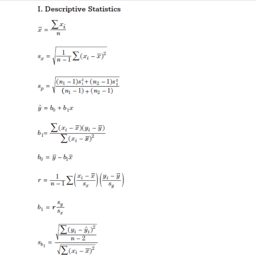
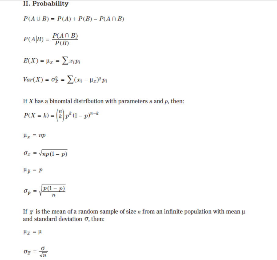
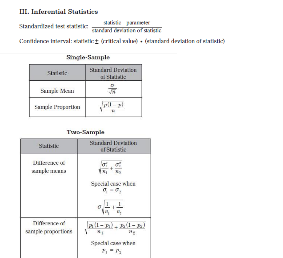
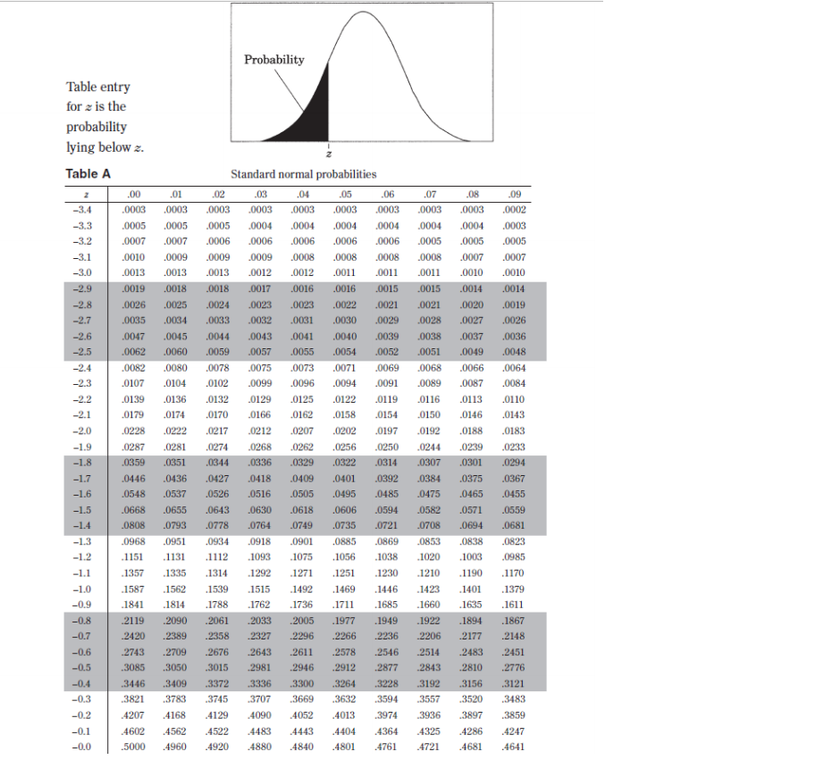
And I attached formula sheet in case you need it for the references.

\fII. Probability P(AUB) = P(A) + P(B) - P(An B) P(AB) = P(An B) P(B) E(X) = Ur = _xiPi Var(X) = 03 = _(x1 - Ux)2 Pi If X has a binomial distribution with parameters n and p, then: P(X = k) = k)p* (1 - p)"-k Hx = np Ox = Vnp(1- p) Hi = P Op = P(1 - p) n If r is the mean of a random sample of size n from an infinite population with mean u and standard deviation o, then: HI = H OF = VnIII. Inferential Statistics Standardized test statistic: statistic - parameter standard deviation of statistic Confidence interval: statistic + (critical value) . (standard deviation of statistic) Single-Sample Statistic Standard Deviation of Statistic Sample Mean Sample Proportion p(1 - p) n Two-Sample Statistic Standard Deviation of Statistic Difference of sample means n2 Special case when 0 =02 Difference of P (1 - PI) + P2 (1 - P2) sample proportions n2 Special case when P = P2Probability Table entry for z is the probability lying below z. Table A Standard normal probabilities .00 .01 .02 .03 -05 .06 07 -08 .09 -3.4 0003 .0003 .0003 0003 0003 .0003 0003 .0003 .0003 .0002 -3.3 .0005 .0005 .0005 0004 .0004 .0004 .0004 0004 0004 .0003 -3.2 .0007 0007 0006 .0006 20006 .0006 0006 .0005 .0005 0005 -3.1 0010 0009 0009 0009 0008 .0008 0008 0008 0007 0007 -3.0 .0013 .0013 -0013 .0012 .0012 .0011 .0011 .0011 .0010 .0010 -2.9 .0019 .0018 .0018 .0017 .0016 .0016 0015 .0015 .0014 .0014 -2.8 .0026 .0025 0024 .0023 0023 .0022 .0021 0021 .0020 .0019 -2.7 .0035 .0034 0033 .0032 .0031 .0030 0029 0028 0027 0026 -2.6 0047 .0045 .0044 .0043 .0041 .0040 .0039 0038 0037 .0036 -2.5 .0062 .0060 .0059 .0057 .0055 .0054 .0052 .0051 .0049 .0048 -2.4 .0082 0080 .0078 .0075 0073 .0071 .0069 0068 -0066 .0064 -2.3 .0107 .0104 .0102 0099 .0096 .0094 0091 .0089 -0087 0084 -2.2 .0139 .0136 .0132 .0129 .0125 0122 .0119 0116 .0113 .0110 -2.1 .0179 .0174 .0170 .0166 .0162 .0158 0154 0150 .0146 0143 -2.0 .0228 .0222 .0217 0212 .0207 .0202 0197 .0192 .0188 0183 -1.9 .0287 .0281 .0274 0268 .0262 .0256 0250 0244 0239 .0233 -1.8 .0359 .0351 .0344 .0336 .0329 .0322 .0314 .0307 ,0301 .0294 -1.7 .0446 .0436 .0427 0418 0409 .0401 0392 .0384 10375 0367 -1.6 .0548 .0537 .0526 0516 -0505 .0495 0485 .0475 .0465 0455 -1.5 .0668 -0655 .0643 0630 _0618 .0606 0594 .0582 .0571 .0559 -1.4 .0808 .0793 0778 .0764 .0749 0735 0721 .0708 10694 0681 -1.3 .0968 .0951 .0934 0918 -0901 .0885 0869 .0853 .0838 0823 -1.2 .1151 .1131 .1112 1093 .1075 1056 1038 .1020 1003 0985 -1.1 .1357 .1335 .1314 .1292 .1271 .1251 1230 .1210 .1190 .1170 -1.0 .1587 1562 .1539 .1515 .1492 .1469 1446 .1423 .1401 .1379 -0.9 .1841 .1814 .1788 1762 .1736 .1711 1685 .1660 .1635 .1611 -0.8 .2119 .2090 2061 2033 .2005 .1977 1949 1922 .1894 .1867 -0.7 .2420 2389 2358 2327 2296 .2266 2236 .2206 .2177 .2148 -0.6 .2743 .2709 .2676 .2643 2611 12578 .2546 .2514 .2483 2451 -0.5 .3085 .3050 3015 2981 2946 2912 .2877 .2843 .2810 .2776 -0.4 .3446 .3409 .3372 .3336 3300 .3264 3228 3192 .3156 .3121 -0.3 .3821 .3783 .3745 .3707 3669 3632 .3594 3557 .3520 3483 -0.2 4207 4168 4129 4090 .4052 4013 3974 3936 3897 .3859 -0.1 4602 4562 4522 4483 4443 .4404 4364 -4325 4286 .4247 -0.0 .5000 .4960 .4920 4880 .4840 .4801 4761 4721 .4681 .4641Probability Table entry for > is the probability lying below z. Table A (Continued) Standard normal probabilities 2 .00 01 .02 .03 .04 .05 .06 .07 .08 -09 0.0 5000 5040 .5080 5120 5160 .5199 5239 5279 -5319 .5359 0.1 5398 .5438 .5478 .5517 .5557 .5596 .5636 .5675 -5714 .5753 0.2 .5793 .5832 .5871 .5910 5948 .5987 6026 .6064 .6103 .6141 0.3 6179 6217 6255 6293 6331 6368 6406 6445 .6480 6517 0.4 6554 6591 6628 6664 6700 6736 6772 6808 6844 6879 0.5 .6915 .6950 6985 .7019 .7054 .7088 .7123 7157 .7190 7224 0.6 7257 7291 7324 7357 7389 .7422 .7454 7486 .7517 .7549 0.7 7580 7611 7642 7673 7704 7734 .7764 7794 7823 17852 0.8 7881 7910 7935 7967 7995 8023 .8051 8078 .8106 .8133 .8159 8186 8212 8238 8264 .8289 8315 8340 8365 .8389 0.9 8461 8485 8508 .8531 .8554 8577 8594 8621 1.0 8413 8438 .8643 8665 8708 8729 8749 8790 8810 1.1 .8770 8830 8686 1.2 8849 8869 8888 690M 8925 .8914 8962 8980 8997 .9015 1.3 9032 9049 9066 9082 9099 .9115 .9131 9147 9162 9177 1.4 9192 9207 9222 9236 .9251 9265 .9279 9292 9306 .9319 1.5 9332 9345 .9357 9370 9382 9394 9406 9418 .9429 .9441 1.6 9452 .9463 .9474 9484 9495 9505 9515 9525 9535 .9545 9554 9564 9573 9582 9591 9599 9608 9616 9625 9633 1.7 9649 9656 9664 .9678 9686 9693 9706 1.8 9641 ,9671 9699 9761 .9767 1.9 9713 .9719 9726 9732 9738 .9714 9750 9756 9812 .9817 20 9772 .977 9783 9788 9793 9798 9803 9808 2.1 9821 19826 9830 9834 9838 9842 9846 9850 .9854 .9857 2.2 9861 .9864 9868 9871 .9875 .9878 9881 9884 .9887 9890 .9896 9901 .9904 9906 .9909 9911 9913 .9916 2.3 .9893 9898 2.4 9918 9920 9922 9925 9927 992 9931 9932 .9934 9936 9938 .9940 9941 9943 .9945 9946 9948 .9949 .9951 .9952 2.5 9953 9959 .9961 9964 9955 995 9957 .9960 9962 .9963 2.6 2.7 .9965 .9966 9967 .9968 .9969 .997 9971 9972 9973 .9974 2.8 .9974 .9975 9976 .9977 .9977 .9978 .9979 .9979 .9980 .9981 .9981 .9982 .9982 9983 19984 .9984 9985 9985 .9986 .9986 2.9 3.0 9987 .9987 4987 9988 9988 9989 9989 9989 9990 .9990 3.1 .9990 .9991 9991 9991 9992 9992 9992 9992 9993 .9993 3.2 .9993 .9993 .9994 9994 .9994 .9994 .9994 .999 .9995 .9995 3.3 .9995 .9995 .9995 9996 9996 .9996 .9996 .9996 9996 .9997 3.4 9997 9997 9997 .9997 9997 9997 .9998 .9997 .9997 .9997Table entry for p and C is the point #* with probability p lying above it Probability p and probability C lying between -t* and * Table B t distribution critical values Tail probability p df .25 .20 -15 10 05 .025 .02 .01 .005 0025 .001 .0005 1.000 1.376 1.963 3.078 6.314 12.71 15.89 31.82 63.66 127.3 318.3 636.6 .816 1.061 1 386 1.886 2.920 4.303 4.849 6.965 9.925 14.09 22.33 31.60 765 .978 1.250 1.638 2.353 3.182 3.482 4.541 5.841 7.453 10.21 12.92 .741 941 1.190 1.533 2.132 2.776 2.999 3.747 4.604 5.598 7.173 8.610 .727 920 1.156 1.476 2.015 2.571 2.757 3.365 4.032 4.773 5.893 6.869 718 906 1.134 1.440 1.943 2.447 2.612 3.143 3.707 4.317 5.208 5.959 .711 896 1.119 1.415 1.895 2.365 2.517 2.948 3.499 4.029 4.785 5.408 .706 1.108 1.397 1.860 2.306 2.449 2.896 3.355 3.833 4.501 5.041 703 883 1.100 1.383 1.833 2.262 2.398 2.821 3.250 3.690 4.297 4.781 10 .700 879 1.093 1.372 1.812 2.228 2.359 2.764 3.169 3.581 4.144 4.587 11 697 876 1.088 1.363 1.796 2.201 2.328 2.718 3.106 3.497 4.025 4.437 873 1.083 1.356 1.782 2.179 2.303 2.681 3.055 3.428 3.930 4.318 1.079 1.350 1.771 2.160 2.282 2.650 3.012 3.372 3.852 4.221 .692 1.076 1.345 1.761 2.145 2.264 2.624 2.977 3.326 3.787 4.140 15 691 1.341 1.753 2.131 2.249 2.612 2.947 3.286 3.733 4.073 16 69 865 1.071 1.337 1.746 2.120 2.235 2.583 2.921 3.252 3.686 4.015 17 .685 LU69 1.333 2.110 2.224 2.567 2.898 3.222 3.646 3.965 18 1067 1.330 1.734 2.101 2.214 2.552 2.878 3.197 3.611 3.922 19 .688 861 1.066 1.328 1.729 2.093 2.205 2.539 2.861 3.174 3.579 3.883 20 687 $60 1.064 1.325 1.725 2.086 2.197 2.528 2.845 3.153 3.552 3.850 21 .686 859 1.063 1.323 1.721 2.080 2.189 2.518 2.831 3.527 3.819 22 .686 858 1.061 1.321 1.717 2.074 2.183 2.508 2.819 3.119 3.505 3.792 23 685 858 1.060 1.319 1.714 2.069 2.177 2.500 2.807 3.104 3.485 3.768 24 .685 857 1.059 1.318 1.711 2.064 2.172 2.492 2.797 3.467 3.745 25 684 356 1058 1.316 1.708 2.060 2.167 2.485 2.787 3.078 3.450 3.725 26 684 856 1058 1.315 1.706 2.056 2.162 2.479 2.779 3.067 3.435 3.707 27 .684 855 1.314 1.703 2.052 2.158 2.473 2.771 3.057 3.421 3.690 28 683 855 1.056 1.313 1.701 2048 2.154 2.467 2.763 3.047 3.408 3.674 29 68 854 1,055 1.311 1.699 2.045 2.150 2.462 2.756 3.038 3.396 3.659 30 .683 854 1.055 1.310 1.697 2.042 2.147 2.457 2.750 3.030 3.385 3.646 40 .681 851 1.050 1.303 1.684 2.123 2.423 2.704 3.307 3.551 50 679 849 1.047 1.299 1.676 2.009 2.109 2.403 2.678 2.937 3.261 3.496 60 679 .848 1.045 1.296 1.671 2.000 2.099 2.390 2.660 2.915 3.232 3.460 80 678 846 1043 1.292 1.664 1.990 2088 2.374 2.639 2.887 3,195 3.416 100 .677 .845 1.042 1.290 1.660 1.984 2.081 2.364 2.626 2.871 3.174 3.390 1000 .675 842 1.037 1.282 1.646 1.962 2.056 2.330 2.581 2.813 3.098 3.300 674 841 1.036 1.282 1.645 1.960 2.054 2.326 2.576 2.807 3,091 3.291 50% 60% 70% 80% 90% 95% 96% 98% 99% 99.5% 99.8% 99.9%%Table entry Probability p for p is the point (x ) with probability p (X ?) lying above it. Table C x critical values Tail probability p .02 01 0025 dif 25 20 .15 -10 .05 1025 005 .001 2.71 3.8 5.02 5.41 6.63 7.8 9.14 10.83 1.32 1.64 2.07 3.79 4.61 5.99 7.38 7.82 921 10.60 1198 13.82 2.77 3.22 6.25 781 9.35 984 11.34 12 84 14 32 16.27 4.11 4.64 5.32 5.39 5.90 6,74 7.78 9.19 11.14 11.67 13 28 14.86 1642 18.47 15.09 18 39 20.51 6.63 8.12 9.24 11.07 12 89 16.75 40.25 22.46 7.84 8.56 9.45 10.64 12.59 14.45 15.03 16.61 18.51 14 07 16.01 16.62 18.48 22.04 24.32 9.04 9.80 10.75 12.02 21.95 23.77 26.12 10.22 11.03 12 03 13.36 15.51 17.53 18.17 20.09 21.67 23.59 25.46 27.88 11.3 13.29 14.68 16.92 19.02 19.68 12.24 23.21 25.19 29.59 12.5 13.44 14.53 18.31 20.48 21.16 27.11 15.99 28.73 31.26 13.70 14.63 15.77 17.28 19.68 21.92 22.62 24.72 26.76 23.34 24.05 26.22 28.30 30.32 32.91 14.85 15.81 16.94 18.55 21.03 22.36 24.74 25.47 27.69 29.82 31.88 34.53 15.98 16.98 18.20 19.81 21.06 23.68 26.12 26.87 29.14 31.32 33.43 36.12 17.12 18.15 19.41 18.25 19.31 20.60 22.31 25.00 27.49 28.26 30.58 32.80 34.95 37.70 20.47 21.79 23.54 26.30 28.85 29.63 32.00 34.27 36.46 39.25 19.37 30.19 31.00 33.41 35.72 37.95 40.79 20.49 21.61 22.98 24.77 27.59 32.35 34.81 37.16 39.42 42.31 21.60 22.76 24.16 25.99 28.87 31.53 22.72 23.90 25.33 27.20 30.14 32.85 33.69 36.19 38.58 40.88 43.82 26.50 28.41 31.41 34.17 35.02 37.57 40.00 12.34 45.31 23.83 25.04 29.62 32.67 35.48 36.34 38.93 41.40 43.78 46.80 24.93 26.17 27.66 26.04 27.30 28.82 30.81 33.92 36.78 37.66 40.29 12 81 45.20 48.27 38 97 41.64 14.18 16 62 49.73 27.14 28.43 29 98 35.17 38.08 39.36 40.27 42.98 45.56 1803 51.18 28 2 2955 31.13 23.20 3642 32.28 14.38 37.65 40.65 41.57 44.31 46.93 29.3 33.43 15.56 38.89 41.92 12 8 45.64 48 2 54.05 26 30.4 31.79 13.15 14.14 46.96 19.6 52.22 55.48 32.91 34.57 36.74 4011 3.1.5 41.34 14.46 45.42 18 28 50.9 53.59 56.89 28 32.6 34.03 35.71 37.92 58.30 16069 19.59 52.3 54.97 33.7 35.14 36.85 39.09 42.56 15.72 34.80 36.25 37.9 40.26 43.77 46.98 47.96 50.89 53.67 56.3 59.70 45.62 47.27 49.24 51.81 55.76 59.34 60.44 63.69 66.77 69.70 73.40 79.49 $2.66 86.66 56.33 58.16 60.35 63.17 67.50 71.42 72.61 76.15 99.61 66.9 68.97 71.34 74.4 79.08 83.30 84.58 8.8.38 91.95 95.34 124.8 80 88.13 90.41 93.11 96.58 101.9 106.6 108.1 112.3 116.3 120.1 140.2 111.7 131.1 149.4 114.7 118.5 129.6 100 124.3 135.8 144.3 109.1D Question 8 10 pts 8. Suppose a law firm has 1,000 across the country, divided equally into teams of 20 workers in each of the 50 states in the United States. The distributions of salaries of these thousand workers has a mean of $65,000 and a standard deviation of $4,500. i. If we randomly select one of the 1,000 workers, what is the probability that person would have a salary between $55,000 and $70,000? Answer: [ Select ] ii. Consider each team of 20 as a random sample. If we look at any one particular team, what is the probability that the mean salary of this team is between $55,000 and $70,000? Answer: [ Select ] [ Select 0.9999 0.9191 0.8536 0.6835 0.3865Question 6 10 pts 6. For each statement, determine whether the the sampling distribution of sample means is approximately normal, skewed, or cannot be determined. i. The population is normal and the sample sizes are 12. [ Select ] Select] normal skewed ii. The population is normal and the sample sizes are 50. cannot be determined iii. The population is skewed right and the sample sizes are 12. [Select ] iv. The population shape is unknown and the sample sizes are 50. [ Select ]D Question 4 10 pts 4. Match the following symbols to their meaning. i. p ii. ac iii. ox [ Choose ] [ Choose standard deviation of sample means sample mean of standard deviations ii. sample proportion population proportion population mean sample mean sample size jii. [ Choose ]D Question 9 10 pts 9. Suppose there are 9000 students in your school district and that the ages of the students are distributed approximately normally with a mean age of 12.5 and a standard deviation of 4.5. i. The teachers will randomly select one student from the entire district to receive a college scholarship of $5,000. What is the probability that this student is at least 15 years old? Answer: [ Select ] ii. Suppose the teachers randomly select a group of 5 students to receive a $1000 scholarship. What is the probability that the mean age of these students is at least 15 years old? Answer: [Select ] iii. Suppose the teachers also randomly select a group of 10 students to receive a $5 gift card to the cafeteria. What is the probability that the mean age of these students is at least 15 years old? Answer: [Select ] [ Select ] 8.3x10^-29 0.0395 0.1071 0.2892 0.9605D Question 1 10 pts 1. A nation wide standardized exam has a mean of 85 and a standard deviation of 10. Suppose that samples of size n = 25 are drawn randomly from all of the scores in the nation. What is the probability that any particular sample has a sample mean between 80 and 90? This question is adapted from from openstaxcollege. org. Download for free at http:/cox.org/contents/30180442-8098-4886-ac05-ed152b@1b0de@18.13p O 0.38 O 0.49 O 0.56 O 0.91 O 0.99 D Question 2 10 pts 2. The time it takes Americans to complete their income tax forms each year is normally distributed with a mean of 5 hours and a standard deviation of 1.5 hours. Which of the following must be true? There may be more than one answer. Select all that apply. The sampling distribution for samples of size 25 has a standard deviation of 0.3 The sampling distribution of size 25 is normally distributed. The probability that a random sample of size 25 has a mean larger than 6.5 hours is 0.45