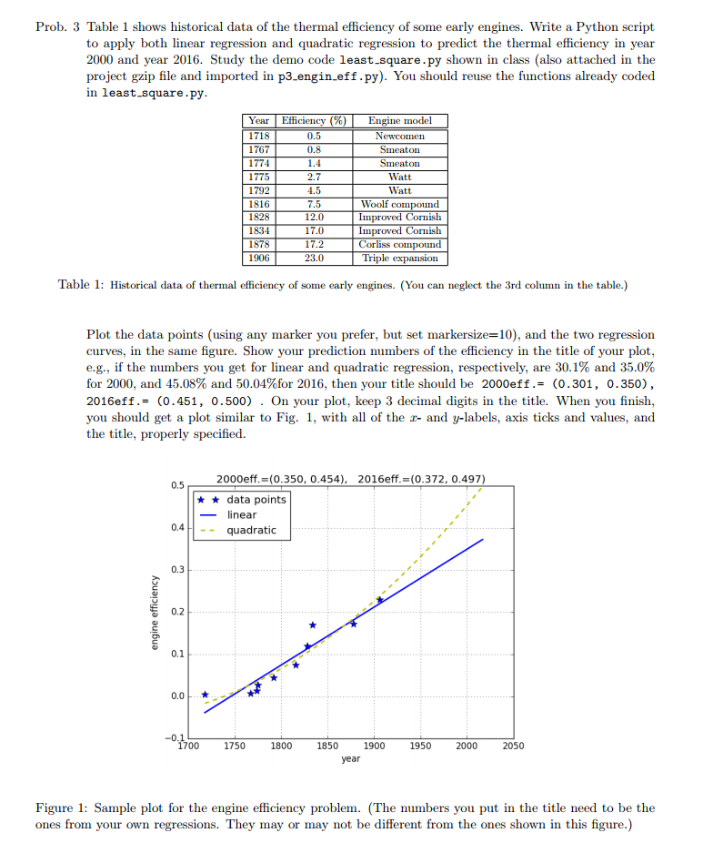
""" This problem asks you to plot data points, then apply linear regression and quadratic regression to predict the engin efficiency in 2000 and 2016, show the predicted numbers in the plot title.

"""

import numpy as np import scipy.linalg as linalg import matplotlib.pyplot as plt import least_square as LS #then call the function least_square_poly() as LS.least_square_poly()

#---------------------------------------------------------- def engin_efficiency(): # # input the data from the table, make them to be np.array so that they can be scaled # xData = yData =

# # call the least_square_poly() for regression #

# print the standard deviation

# plot your data points

# plot linear regression line

# plot quadratic regression curve

# set the labels and lengends etc

# # find the predicted values that are for years 2000 and 2016, set the title properly #

plt.savefig("engin_efficiency.png") plt.show()

Here is the leastsquare py file code.

## module least square fitting

import numpy as np import scipy.linalg as linalg

def least_square_poly(xData, yData, m, x): ''' least square fit (xData, yData) using a degree m polynomial, return the polynomial evaluated at x, where x can be a list or an numpy array. ''' # #make sure the input arrays are np.array (instead of lists) so that they can be scaled # xData=np.array(xData); yData=np.array(yData); x=np.array(x)

# ##construct the Vandermonde matrix (vectorized version, using just one loop) # n = len(xData) A = np.empty((n, m+1)) A[:,0]=np.ones(n) for i in range(1, m+1): A[:,i] = A[:,i-1] * xData

# ##call the lstsq function in scipy to solve for the least square solution (the coefficient vector c) # c, resid, rank, sigma = linalg.lstsq(A, yData)

# ##polynomial evaluation p(x)=c[0]+c[1]*x + ...+c[m]*x**m # return eval_poly(c, x), stDev(c, xData, yData)

def eval_poly(c, x): ''' evaluation the polynomial p(x)=c[0]+c[1]*x + ...+c[m]*x**m, the polynomial degree is automatically detected by the length of the coefficient vector c. ''' m = len(c)-1 p = c[m] for i in range(m, 0, -1): p = x*p + c[i-1] return p

def stDev(c, xData, yData): ''' compute standard deviation ''' px = eval_poly(c, xData) sigma = np.linalg.norm(px - yData, 2) return sigmap.sqrt(len(xData) - len(c))

#################################################################### if __name__=='__main__':

import matplotlib.pyplot as plt

# # show lower degree polynomial fitting of data from a higher order polynomial # # 1. polynomial curve n = 10; xmax=2; xstep = 0.2 xData = np.arange(0, xmax, xstep) f = lambda x : 1 + x + x**2/5 + x**3/20 + x**4/100 + x**20/1000 perturb=4.0 #set perturb=0 to see exact polynomial match yData = f(xData) + perturb*np.random.randn(np.size(xData))

xv = np.arange(0, xmax-xstep+.01, 0.04) mmax = 7 px = np.empty((len(xv), mmax-1)); stdLS={} for m in range(1,mmax): px[:,m-1], stdLS[m-1] =least_square_poly(xData, yData, m, xv) #print("px[:, {}]={}".format(m-1, px[:,m-1]))

print(stdLS)

fig1 = plt.plot(xv, f(xv), 'b:', xData, yData, '*', xv, px[:,0], 'b-', xv, px[:,1], 'y--', xv, px[:,2], 'c-.', xv, px[:,3], 'k--', xv, px[:,4], 'r-', xv, px[:,5], 'r:') plt.legend(('exact poly.', 'data points', 'linear', 'quadratic', 'cubic', '4th order', '5th order', '6th order'), loc="best") plt.xlabel("x, (data perturb={})".format(perturb)) plt.show()

# 2. show lower degree polynomial fitting of data from a non polynomial curve n = 12; xmax=10; xstep = 0.5 xData = np.arange(0, xmax, xstep) fe = lambda x : 1 + x + np.exp(x)*np.sin(x) perturb=0.0 # yData = fe(xData) + perturb*np.random.randn(np.size(xData))

xv = np.arange(0, xmax-xstep+.01, 0.05) mmax = 7 px = np.empty((len(xv), mmax-1)); stdLS={} for m in range(1,mmax): px[:,m-1], stdLS[m-1]=least_square_poly(xData, yData, m, xv) #print("px[:, {}]={}".format(m-1, px[:,m-1]))

print(stdLS) plt.plot(xv, fe(xv), 'b--', lw=1.5, label='exact funct') plt.plot(xData, yData, '*', markersize=10, label="data points") plt.plot(xv, px[:,0], 'b-', lw=2, label="linear") plt.plot(xv, px[:,1], 'y--', lw=2, label="quadratic") plt.plot(xv, px[:,2], 'c-.', lw=2.5, label="cubic") plt.plot(xv, px[:,3], 'k--', lw=2.5, label="4th order") plt.plot(xv, px[:,4], 'y-', lw=2, label="5th order") plt.plot(xv, px[:,5], 'r-', lw=2, label="6th order") #plt.legend(('exact funct', 'data points', 'linear', 'quadratic', 'cubic', '4th order', # '5th order', '6th order'), loc="best") plt.legend(loc="best") plt.xlabel("x, (data perturb={})".format(perturb)) plt.show()

Prob. 3 Table 1 shows historical data of the thermal efficiency of some early engines. Write a Python script to apply both linear regression and quadratic regression to predict the thermal efficiency in year 2000 and year 2016. Study the demo code least.square.py shown in class (also attached in the project gzip file and imported in p3 engin.eff.py). You should reuse the functions already coded in least.square.py Engine model Newcomen Smeaton Smeaton Watt Watt 1718 1767 1774 0.5 0.8 1792 1816 1828 1834 1878 1906 2.7 4.5 7.5 12.0 17.0 17.2 23.0 nd Cornish Woolf com Corliss comp Triple expansion Table 1: Historical data of thermal efficiency of some early engines. (You can neglect the 3rd column in the table.) Plot the data points (using any marker you prefer, but set markersze=10), and the two regression curves, in the same figure. Show your prediction numbers of the efficiency in the title of your plot, eg, if the numbers you get for linear and quadratic regression, respectively, are 30.1% and 35.0% for 2000, and 45.08% and 50.04%for 2016, then your title should be 2000eff .= (0.301, 0.350) , 2016eff.= (0.451, 0.500) . On your plot, keep 3 decimal digits in the title. When you finish. you should get a plot similar to Fig. 1, with all of the x- and y-labels, axis ticks and values, and the title, properly specified. 2000eff.=(0.350,0.454), 2016eff.=(0.372,0.497) 0.5 data points linear 0.4Hquadratioc 0.3 0.2 0.0L -0 1750 1800 1850 1900 1950 2000 2050 year Figure 1: Sample plot for the engine efficiency problem. (The numbers you put in the title need to be the ones from your own regressions. They may or may not be different from the ones shown in this figure.)