Tiffany owns an event management business that is currently operating from her garage. She would like to transform her guest room into a home office. However, she does not have her own capital to invest and will need to raise $10,000 to renovate and refit the room.
13
Tiffany is considering taking a loan for the required amount for her renovation. Her local bank charges 7.8% per year compounded quarterly and requires quarterly repayments. The bank offered Tiffany a one-year interest-only option with her three-year loan. This means that for the first year, every quarter Tiffany would pay only interest on the amount borrowed. Loan repayments consisting of both interest and principal would then commence in the second year continues for the third year.
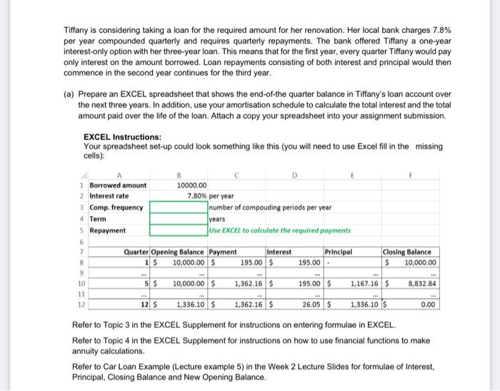
(a) Prepare an EXCEL spreadsheet that shows the end-of-the quarter balance in Tiffanys loan account over the next three years. In addition, use your amortisation schedule to calculate the total interest and the total amount paid over the life of the loan. Attach a copy your spreadsheet into your assignment submission.
EXCEL Instructions:
Your spreadsheet set-up could look something like this (you will need to use Excel fill in the missing cells):
Refer to Topic 3 in the EXCEL Supplement for instructions on entering formulae in EXCEL.
Refer to Topic 4 in the EXCEL Supplement for instructions on how to use financial functions to make annuity calculations.
Refer to Car Loan Example (Lecture example 5) in the Week 2 Lecture Slides for formulae of Interest, Principal, Closing Balance and New Opening Balance.
(b) A wealthy family friend nicknamed Lecce had offered to help Tiffany and has made an alternative offer for her to obtain the $10,000 loan. Lecce has proposed the following loan terms over a 12-month period. He claims this is a cheaper and simple with everything paid off at the end of the renovation.
Lecce will give her the $10,000 at the start of the month and Tiffany will start pay $900 at the each of each month for until the end of the loan period. He claims he is entitled to $800 in interest, which will be paid to him under his proposed conditions.
Tiffany would like to know the interest rate Lecce is charging her and they would also like to verify the total amount of interest ($800) he claims he is entitled to.
To answer this question, follow all EXCEL instructions below including the instructions given in the two diagrams. Also show your calculation for the total interest Tiffany paid under this arrangement.
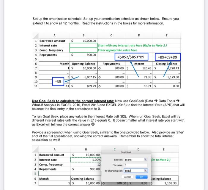
EXCEL Instructions: you will need to set up a new Amortisation schedule, like the one shown below, for the 12-month loan. For full marks provide: (i) a copy of your Excel spreadsheet that looks similar to the one below and (ii) your calculation for the total interest to verify Lecces $800 claim.
14
Set up the amortisation schedule: Set up your amortisation schedule as shown below. Ensure you extend it to show all 12 months. Read the instructions in the boxes for more information.
Use Goal Seek to calculate the correct interest rate: Now use GoalSeek (DataData Tools What-If Analysis in EXCEL 2010, Excel 2013 and EXCEL 2016) to find the Interest Rate (APR) that will balance the final entry in the spreadsheet to 0.
To run Goal Seek, place any value in the Interest Rate cell (B2). When run Goal Seek, Excel will try different interest rates until the value in E18 equals 0. It doesnt matter what interest rate you start with, as Excel will tell you the correct answer J
Provide a screenshot when using Goal Seek, similar to the one provided below. Also provide an after shot of the full spreadsheet, showing the correct answers. Remember to show the total interest calculation as well!
(c) Tiffanyisseekingyouradviceinmakingthisfinancialdecision.Writeashortsummary(8-10sentences, double spaced, at least 2cm margins, 12pt Times New Roman font or equivalent) for the couple explaining your findings.
Set up the amortisation schedule: Set up your amortisation schedule as shown below. Ensure you extend it to show all 12 months. Read the instructions in the boxes for more information B D E 1 Borrowed amount $ 10,000.00 2 Interest rate start with any interest rate here (Refer to Note 2.) 3 Comp. frequency Enter appropriate value here 4 Repayments $ 900.00 5 =$B$2/$B$3*B9 =B9+C9+D9 6 Month Opening Balance Repayments Interest Closing Balance 7 1 S 10,000.00 $ 900.00 $ 120.43S 1,220.43 8 9 6 $ 6,007.15$ 900.00 $ 72.35 $ 5,179.50 10 =E8 11 12 $ 889.29 S 900.00 10.71 S 0.00 Use Goal Seek to calculate the correct interest rate: Now use GoalSeek (Data Data Tools What-lf Analysis in EXCEL 2010, Excel 2013 and EXCEL 2016) to find the Interest Rate (APR) that will balance the final entry in the spreadsheet to 0. To run Goal Seek, place any value in the Interest Rate cell (B2). When run Goal Seek, Excel will try different interest rates until the value in E18 equals O. It doesn't matter what interest rate you start with, as Excel will tell you the correct answer Provide a screenshot when using Goal Seek, similar to the one provided below. Also provide an 'after shot of the full spreadsheet, showing the correct answers. Remember to show the total interest calculation as well! E 1 Borrowed amount 2. Interest rate 3 Comp. frequency 4 Repayments fer to Note 2.) Goal Seek 10,000.00 1.00% Set cells ses18 12 To value o $ 900.00 By changing colt 5082 Cancel Opening Balance 1 $ 10,000.00 5 900.00 5 OM 6 Month 7 losing Balance 8.33 $ 9,108.33 Tiffany is considering taking a loan for the required amount for her renovation. Her local bank charges 7.8% per year compounded quarterly and requires quarterly repayments. The bank offered Tiffany a one-year interest-only option with her three-year loan. This means that for the first year, every quarter Tiffany would pay only interest on the amount borrowed. Loan repayments consisting of both interest and principal would then commence in the second year continues for the third year. (a) Prepare an EXCEL spreadsheet that shows the end-of-the quarter balance in Tiffany's loan account over the next three years. In addition, use your amortisation schedule to calculate the total interest and the total amount paid over the life of the loan. Attach a copy your spreadsheet into your assignment submission EXCEL Instructions: Your spreadsheet set-up could look something like this (you will need to use Excel fill in the missing cells): B 1 Borrowed amount 10000.00 2 Interest rate 7.80% per year 3 Comp. frequency number of compouding periods per year 4 Term years 5 Repayment Use EXCEL to calculate the required payments 6 7 Quarter Opening Balance Payment Interest Principal Closing Balance 8 1 $ 10,000.00 $ 195.00 $ 195.00 $ 10,000.00 9 10 5$ 10,000.00 1,362.16 $ 195.00 S 1,167.16 S 8,832.84 12 12 $ 1,336,10 $ 1,362.16 S 26.05 $ 1,336.10 0.00 Refer to Topic 3 in the EXCEL Supplement for instructions on entering formulae in EXCEL. Refer to Topic 4 in the EXCEL Supplement for instructions on how to use financial functions to make annuity calculations. Refer to Car Loan Example (Lecture example 5) in the Week 2 Lecture Slides for formulae of Interest, Principal, Closing Balance and New Opening Balance. Set up the amortisation schedule: Set up your amortisation schedule as shown below. Ensure you extend it to show all 12 months. Read the instructions in the boxes for more information B D E 1 Borrowed amount $ 10,000.00 2 Interest rate start with any interest rate here (Refer to Note 2.) 3 Comp. frequency Enter appropriate value here 4 Repayments $ 900.00 5 =$B$2/$B$3*B9 =B9+C9+D9 6 Month Opening Balance Repayments Interest Closing Balance 7 1 S 10,000.00 $ 900.00 $ 120.43S 1,220.43 8 9 6 $ 6,007.15$ 900.00 $ 72.35 $ 5,179.50 10 =E8 11 12 $ 889.29 S 900.00 10.71 S 0.00 Use Goal Seek to calculate the correct interest rate: Now use GoalSeek (Data Data Tools What-lf Analysis in EXCEL 2010, Excel 2013 and EXCEL 2016) to find the Interest Rate (APR) that will balance the final entry in the spreadsheet to 0. To run Goal Seek, place any value in the Interest Rate cell (B2). When run Goal Seek, Excel will try different interest rates until the value in E18 equals O. It doesn't matter what interest rate you start with, as Excel will tell you the correct answer Provide a screenshot when using Goal Seek, similar to the one provided below. Also provide an 'after shot of the full spreadsheet, showing the correct answers. Remember to show the total interest calculation as well! E 1 Borrowed amount 2. Interest rate 3 Comp. frequency 4 Repayments fer to Note 2.) Goal Seek 10,000.00 1.00% Set cells ses18 12 To value o $ 900.00 By changing colt 5082 Cancel Opening Balance 1 $ 10,000.00 5 900.00 5 OM 6 Month 7 losing Balance 8.33 $ 9,108.33 Tiffany is considering taking a loan for the required amount for her renovation. Her local bank charges 7.8% per year compounded quarterly and requires quarterly repayments. The bank offered Tiffany a one-year interest-only option with her three-year loan. This means that for the first year, every quarter Tiffany would pay only interest on the amount borrowed. Loan repayments consisting of both interest and principal would then commence in the second year continues for the third year. (a) Prepare an EXCEL spreadsheet that shows the end-of-the quarter balance in Tiffany's loan account over the next three years. In addition, use your amortisation schedule to calculate the total interest and the total amount paid over the life of the loan. Attach a copy your spreadsheet into your assignment submission EXCEL Instructions: Your spreadsheet set-up could look something like this (you will need to use Excel fill in the missing cells): B 1 Borrowed amount 10000.00 2 Interest rate 7.80% per year 3 Comp. frequency number of compouding periods per year 4 Term years 5 Repayment Use EXCEL to calculate the required payments 6 7 Quarter Opening Balance Payment Interest Principal Closing Balance 8 1 $ 10,000.00 $ 195.00 $ 195.00 $ 10,000.00 9 10 5$ 10,000.00 1,362.16 $ 195.00 S 1,167.16 S 8,832.84 12 12 $ 1,336,10 $ 1,362.16 S 26.05 $ 1,336.10 0.00 Refer to Topic 3 in the EXCEL Supplement for instructions on entering formulae in EXCEL. Refer to Topic 4 in the EXCEL Supplement for instructions on how to use financial functions to make annuity calculations. Refer to Car Loan Example (Lecture example 5) in the Week 2 Lecture Slides for formulae of Interest, Principal, Closing Balance and New Opening Balance


