To answer these questions, you will need to read Chapter 9, Market Equilibrium & Product Price - Imperfect Competition and please good Good format.

#.Explain the 3 types of "Imperfect" market structures used in selling goods. For each type of market structure, give an agricultural example.

2.Explain the concept of "entry barriers". What are some examples of entry barriers seen in agricultural business? Which type of market structure most often uses entry barriers to limit competition?

3.Explain the difference between "Monopolistic Competition" and "Perfect Competition". Why would an agricultural producer choose to become a monopolistic competitor?

4.What is an agricultural cooperative? What are the benefits of belonging to an Agricultural Cooperative for a farmer? Explain the Capper-Volstead Act and how it impacts farmers involved in cooperatives.

5.How does the Federal Trade Commission discourage the formation of monopolies? What are 3 key regulatory measures that the FTC can utilize to discourage monopolists in addition to legislative acts.

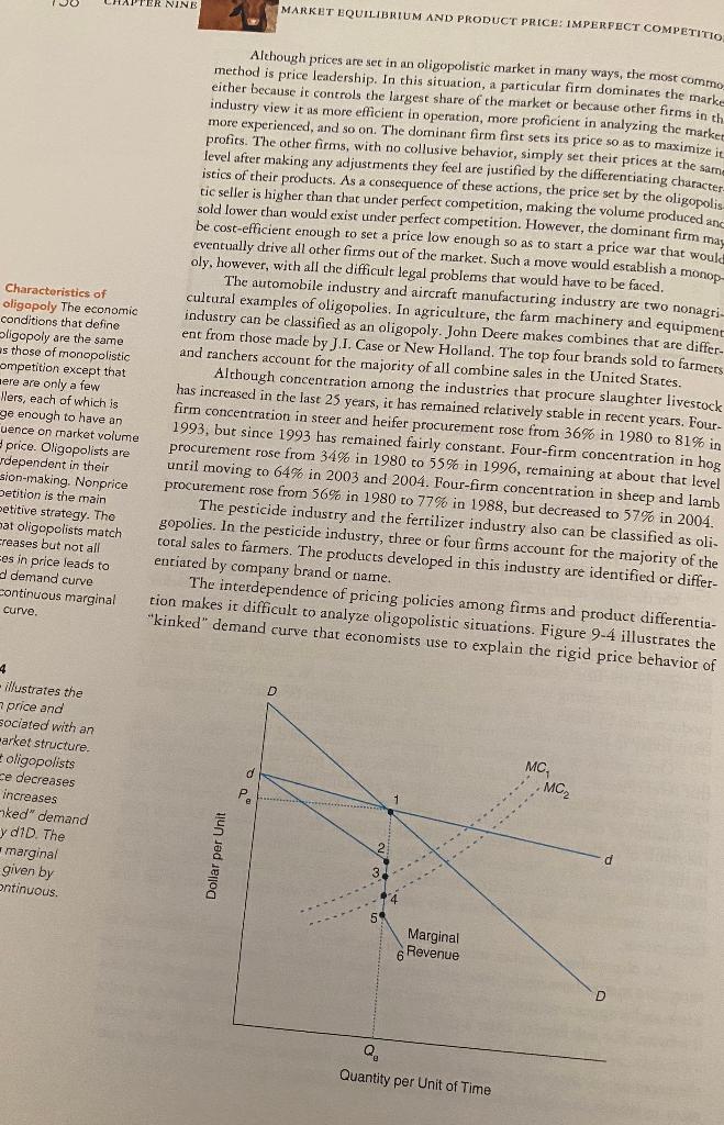
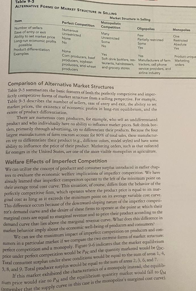
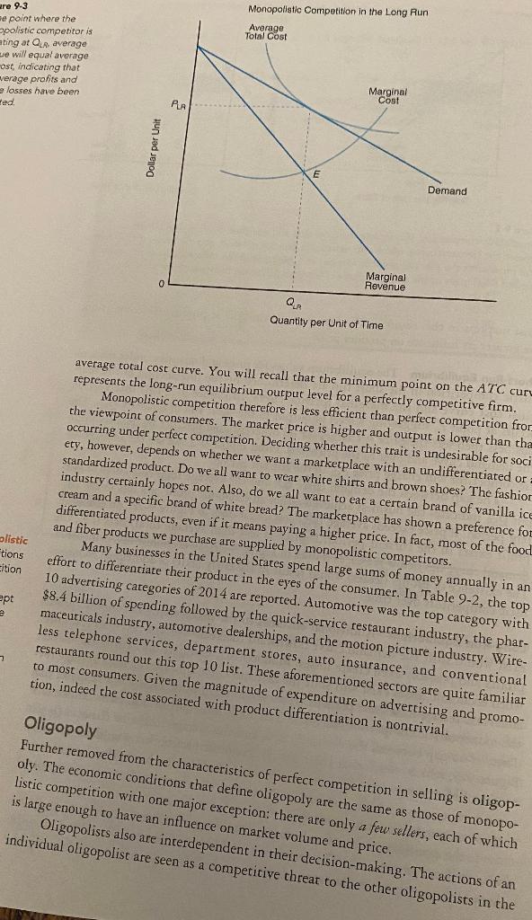
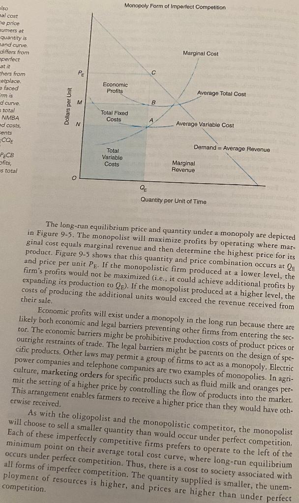
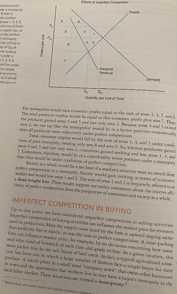
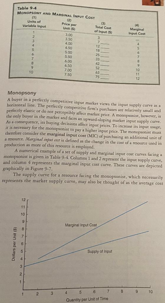
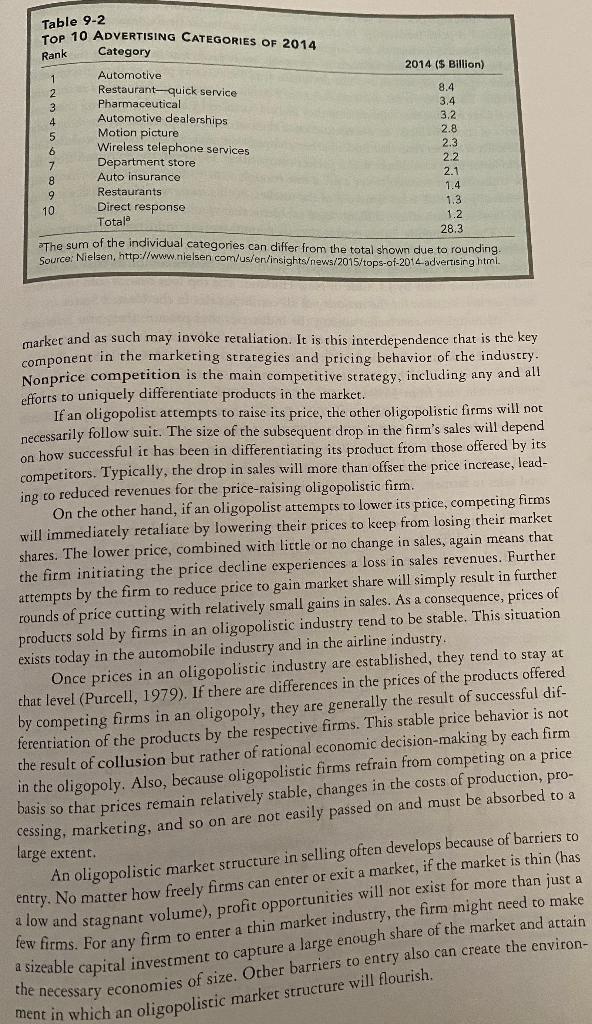
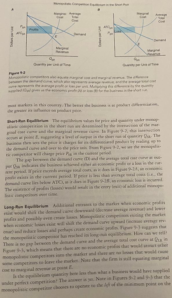
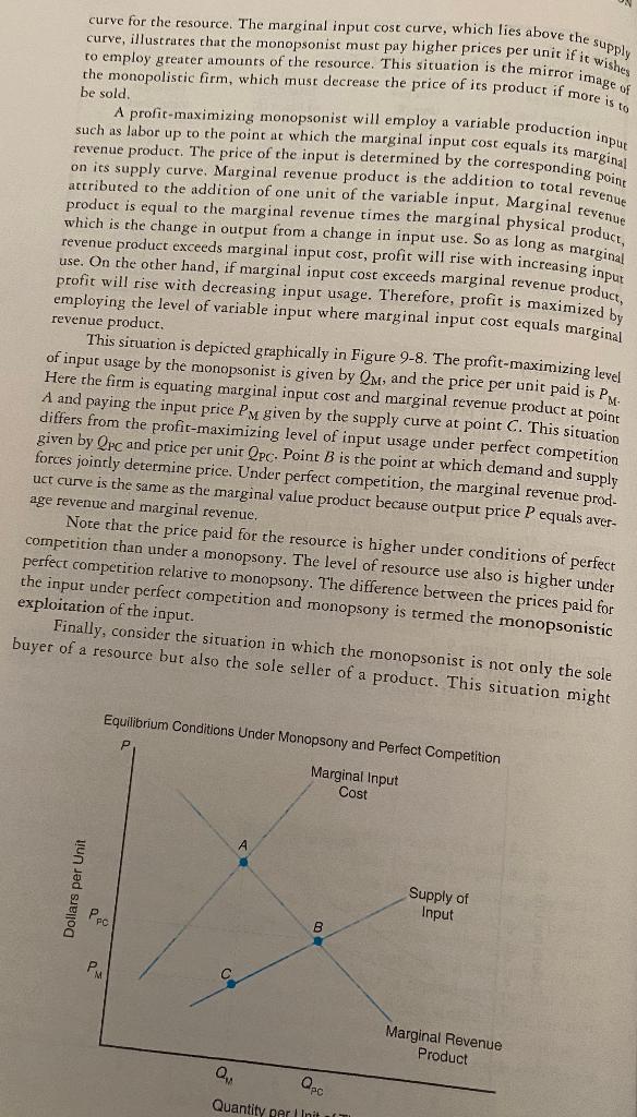
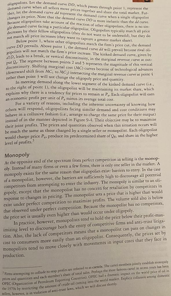
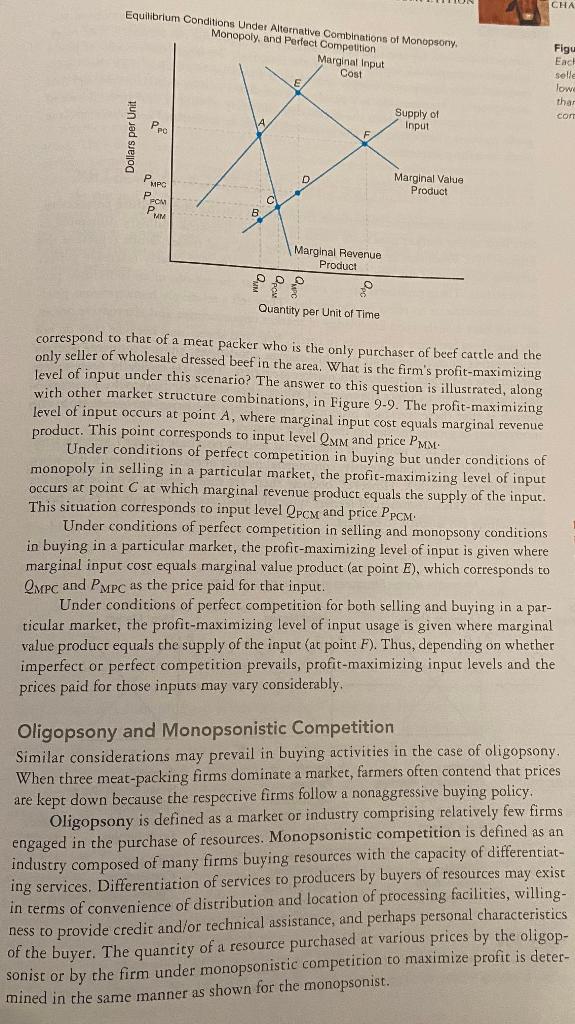
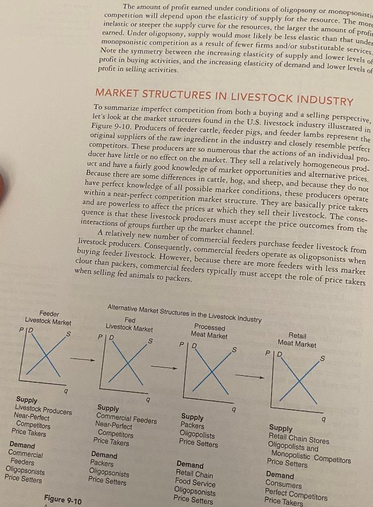
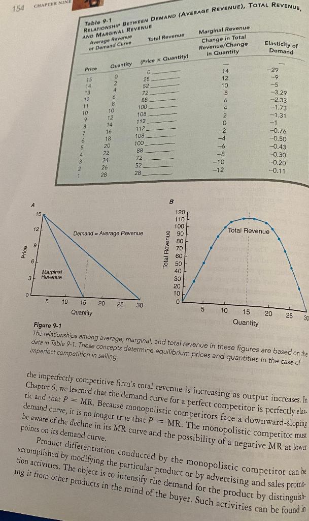
NINE MARKET EQUILIBRIUM AND PRODUCT PRICE: IMPERFECT COMPETITIO COSE Characteristics of oligopoly The economic conditions that define ligopoly are the same as those of monopolistic competition except that aere are only a few Ners, each of which is ge enough to have an uence on market volume price. Oligopolists are dependent in their sion-making. Nonprice Detition is the main setitive strategy. The oligopolists match creases but not all ces in price leads to a demand curve continuous marginal curve. Although prices are set in an oligopolistic market in many ways, the most commo method is price leadership. In this situation, a particular firm dominates the marke either because it controls the largest share of the market or because other firms in th industry view t as more efficient in operation, more proficient in analyzing the marke more experienced, and so on. The dominant firm first sets its price so as to maximize profits. The other firms, with no collusive behavior, simply set their prices at the same level 1 after making any adjustments they feel are justified by the differentiating character istics of their products. As a of these accions, the price set by the oligopolis tic seller is higher than that under perfect competition, making the volume produced an sold lower than would exist under perfect competition. However, the dominant firm may eventually drive all other firms out of the markets such as to start a price war that would move would establish a monop oly, however, with all the difficult legal problems that would have to be faced. The automobile industry and aircraft manufacturing industry are two nonagri- cultural examples of oligopolies. In agriculture, the farm machinery and equipment industry can be classified as an oligopoly. John Deere makes combines that are differ- ent from those made by J.I. Case or New Holland. The top four brands sold to farmers and ranchers account for the majority of all combine sales in the United States. Although concentration among the industries that procure slaughter livestock has increased in the last 25 years, it has remained relatively stable in recent years. Four- firm concentration in steer and heifer procurement rose from 36% in 1980 to 81% in 1993, but since 1993 has remained fairly constant. Four-firm concentration in hog procurement rose from 34% in 1980 to 55% in 1996, remaining at about that level until moving to 64% in 2003 and 2004. Four-firm concentration in sheep and lamb procurement rose from 56% in 1980 to 77% in 1988, but decreased to 57% in 2004. The pesticide industry and the fertilizer industry also can be classified as oli- gopolies. In the pesticide industry, three or four firms account for the majority of the total sales to farmers. The products developed in this industry are identified or differ- entiated by company brand or name. The interdependence of pricing policies among firms and product differentia- tion makes it difficult to analyze oligopolistic situations. Figure 9-4 illustrates the "kinked" demand curve that economists use to explain the rigid price behavior of at 4 D MC, d -illustrates the 7 price and sociated with an -arket structure oligopolists ce decreases increases -ked" demand y did. The marginal given by ontinuous MC Dollar per Unit d Marginal 6 Revenue QA Quantity per Unit of Time Table 9-3 Item ALTERNATIVE FORMS OF MARKET STRUCTURE IN SELLING Market Structure in Selling Monopolistic Competition Oligopolies Number of sellers Numerous Unrestricted Many Ease of entry or exit Few Unrestricted Ability to set market price None Partially restricted Some Long-run economic profits No Some No Yes Perfect Competition Monopolies One Restricted Absolute Yes possible Product differentiation Examples None Com producers, beef producers, soybean producers, and wheat producers Yes Yes Soft drink bottlers, res- Manufacturers of farm taurants, hairdressers, tractors, cell phone and grocery stores service providers, and airline industry Product unique Marketing orders Comparison of Alternative Market Structures Table 9-3 summarizes the basic features of both the perfectly competitive and imper- fectly competitive forms of market structure from a selling perspective. For example, Table 9-3 describes the number of sellers, ease of entry and exit, the ability to set market prices, the existence of economic profits in long-run equilibrium, and the extent of product differentiation. There are numerous corn producers, for example, who sell an undifferentiated product and who individually have no ability to influence market prices. Soft drink bot- tlers, primarily through advertising, try to differentiate their products. Because the four largest manufacturers of farm tractors account for 80% of total sales, these manufactur- ers try to differentiate their product (e.g., different colors, model styles) and have some ability to influence the price of their product. Marketing orders, such as that enforced for oranges in the United States, are one of the more visible monopolies in agriculture. Welfare Effects of Imperfect Competition We can utilize the concept of producer and consumer surplus introduced in earlier chap- ters to evaluate the economic welfare implications of imperfect competition. We have already learned that imperfect competitors operace to the left of the minimum point on their average total cost curve. This situation, of course, differs from the behavior of the perfectly competitive firm, which operates where the product price is equal to its mar- ginal cost as long as it exceeds the minimum point on its average variable cost curve. This difference occurs because of the downward-sloping nature of the imperfect competi- tor's demand curve and the desire of these firms to operate at the point at which their marginal costs are equal to marginal revenue and to price their product according to the demand curve that lies above the marginal revenue curve. What does this difference in market behavior imply about the economic well-being of producers and consumers? We can see the maximum impact of imperfect competition on producers and con- sumers in a particular market if we compare the two extreme forms of market structure: perfect competition and a monopoly. Figure 9-6 indicates that the market equilibrium price under perfect competition would be Ppc and the quantity marketed would be Qpc. Total consumer surplus under these conditions would be equal to the sum of areas 1, 4, 5,8, and 9. Total producer surplus would be equal to the sum of areas 2, 3, 6, and 7. If this market exhibited the characteristics of a monopoly instead, the equilib- fium price would rise to Px and the equilibrium quantity market would fall to em (remember that the supply curve in this case is the monopolist's marginal cost curve). are 9-3 Monopolistic Competition in the Long Run Average Total Cost e point where the poolistic competitor is ating at QA average ele will equal average ost, indicating that werage profits and e losses have been ted Marginal Cost ALA Dollar per Demand Marginal Revenue QA Quantity per Unit of Time olistic tions ition average total cost curve. You will recall that the minimum point on the ATC cur represents the long-run equilibrium output level for a perfectly competitive firm. Monopolistic competition therefore is less efficient than perfect competition from the viewpoint of consumers. The market price is higher and output is lower than tha occurring under perfect competition. Deciding whether this trait is undesirable for soci ety, however, depends on whether we want a marketplace with an undifferentiated or standardized product. Do we all want to wear white shirts and brown shoes? The fashion industry certainly hopes not. Also, do we all want to eat a certain brand of vanilla ice cream and a specific brand of white bread? The marketplace has shown a preference for differentiated products, even if it means paying a higher price. In fact, most of the food and fiber products we purchase are supplied by monopolistic competitors. Many businesses in the United States spend large sums of money annually in an effort to differentiate their product in the eyes of the consumer. In Table 9-2, the top 10 advertising categories of 2014 are reported. Automotive was the top category with $8.4 billion of spending followed by the quick-service restaurant industry, the phar- maceuticals industry, automotive dealerships, and the motion picture industry. Wire- less telephone services, department stores, auto insurance, and conventional restaurants round out this top 10 list. These aforementioned sectors are quite familiar to most consumers. Given the magnitude of expenditure on advertising and promo- tion, indeed the cost associated with product differentiation is nontrivial. Oligopoly Ept 7 Further removed from the characteristics of perfect competition in selling is oligop- oly. The economic conditions that define oligopoly are the same as those of monopo- Listic competition with one major exception: there are only a few sellers, each of which is large enough to have an influence on market volume and price. Oligopolists also are interdependent in their decision-making. The actions of an individual oligopolist are seen as a competitive threat to the other oligopolists in the DIE Monopoly Form of Imperfect Competition lso al cost he price sumers at quantity is mand curve differs from perfect Marginal Cost at it Pe thers from etplace. e faced Erm is Economic Profits Average Total Cost d curve total NMBA ed costs, Dollars per Unit Total Fixed Costs A N Average Variable Cost tents COE Demand = Average Revenue Ofits, 15 total Total Variable Costs Marginal Revenue QE Quantity per Unit of Time The long-run equilibrium price and quantity under a monopoly are depicted in Figure 9-5. The monopolist will maximize profits by operating where mar- ginal cost equals marginal revenue and then determine the highest price for its product. Figure 9-5 shows that this quantity and price combination occurs at Qe and price per unit Pe. If the monopolistic firm produced at a lower level, the firm's profits would not be maximized (i.e., it could achieve additional profits by expanding its production to Qe). If the monopolist produced at a higher level, the costs of producing the addicional units would exceed the revenue received from their sale. Economic profits will exist under a monopoly in the long run because there are likely both economic and legal barriers preventing other firms from entering the sec- tor. The economic barriers might be prohibitive production costs of product prices or outright restraints of trade. The legal barriers might be patents on the design of spe- cific products. Other laws may permit a group of firms to act as a monopoly. Electric power companies and telephone companies are two examples of monopolies. In agri- culture, marketing orders for specific products such as fluid milk and oranges per- mit the setting of a higher price by controlling the flow of products into the market. This arrangement enables farmers to receive a higher price than they would have oth- erwise received. As with the oligopolist and the monopolistic competitor, the monopolist will choose to sell a smaller quantity than would occur under perfect competition Each of these imperfectly competitive firms prefers to operate to the left of the minimum point on their average total cost curve, where long-run equilibrium occurs under perfect competition. Thus, there is a cost to society associated with all forms of imperfect competition. The quantity supplied is smaller, the unem- ployment of resources is higher, and prices are higher than under perfect competition Effects of Imperfect Competition Supply 9 8 PM 5 4 1 surplus would der a monopoly 9) than it der perfect areas 1,4,58 cers would have o supply Opc at under perfect a monopoly, be willing to ity of Quat acer surplus runder a = 3, 4, 5, 6, -uld be under Fion (areas PC 32 Dollars per Unit 6 7 Marginal Revenue e economic - as a whole Demand the sum of Q Opc Quantity per Unit of Time The monopolist would earn economic profits equal to the sum of areas 3, 4, 5, and 6. The total producer surplus would be equal to this economic profit plus area 7. Thus, the producer gained areas 4 and 5 and lost only area 2. Because areas 4 and 5 exceed area 2, we can say that the monopolist would be in a better position economically than all producers were collectively under perfect competition. Total consumer surplus would fall by the sum of areas 1, 4, and 5 under condi- tions of pure monopoly, totaling only area 8 and area 9. So, whereas producers gained areas 4 and 5 and lost only area 2, consumers gained nothing and lost areas 1, 4, and 5. Consumers, therefore, would be in a considerably worse position under a monopoly than they would be under conditions of perfect competition. Society as a whole would be a net loser if a market's structure were to switch from perfect competition to a monopoly. Society would gain nothing in terms of economic welfare and would lose areas 1 and 2. The sum of areas 1 and 2 is frequently referred to as a dead-weight loss. These results support our earlier statements about the relative effi- ciency of perfect competition from the perspective of consumers and society as a whole. IMPERFECT COMPETITION IN BUYING Up to this point, we have considered imperfect competition in selling activities. Imperfect competition in buying activities can influence the market price for resources used in production. Here the supply curve faced by the firm is upward sloping rather than perfectly flat or elastic, as was the case in perfect competition. A meat-packing firm can influence market price, for example, by its decisions concerning how and what kind of livestock of each class and grade to buy. In a given location, this meat packer may be the only buyer of beef cattle. In fact, a typical agricultural situa- tion has been one in which a large number of farmers face a single buyer for their product. A textile plant in a small rural "company town" that owns other businesses in town and the apartments that workers live in may have a buyer's monopoly in the local labor market. These situations are termed a monopsony. any * Where there are several buyers in a similar situation, oligopro Table 9.4 Price per Unit (5) (4) Marginal Input Cost MONOPSONY AND MARGINAL INPUT COST (1) (2) Units of 13) Total Cost Variable Input of Input (5) 3 3.00 2 3 3.50 7 3 4.00 12 4 4.50 18 5 5.00 25 6 5.50 33 7 6.00 42 a 6.50 52 9 7.00 63 10 7.50 75 4 5 6 7 8 9 10 11 12 Monopsony A buyer in a perfectly competitive input market views the input supply curve as a horizontal line. The perfectly competitive firm's purchases are relatively small and perfectly elastic or do not perceptibly affect market price. A monopsonist, however, is the only buyer in the market and faces an upward-sloping market input supply curve. As a consequence, its buying decisions affect input prices. To increase its input usage, it is necessary for the monopsonist to pay a higher input price. The monopsonist must therefore consider the marginal input cost (MIC) of purchasing an additional unit of a resource. Marginal input cost is defined as the change in the cost of a resource used in production as more of this resource is employed. A numerical example of a set of supply and marginal inpur cost curves facing a monopsonist is given in Table 9-4. Columns 1 and 2 represent the input supply curve, and column 4 represents the marginal input cost curve. These curves are depicted graphically in Figure 9-7. The supply curve for a resource facing the monopsonist, which necessarily represents the market supply curve, may also be thought of as the average cost 12 11 10 9 Marginal Input Cost 18 7 Dollars per Unit ($) 6 Supply of Input 2 1 9 8 3 1 10 2 4 5 6 7 Quantity per Unit of Time Table 9-2 Rank TOP 10 ADVERTISING CATEGORIES OF 2014 Category 2014 ($ Billion) 1 Automotive 2 8.4 Restaurant-quick service 3 Pharmaceutical 3.4 4 3.2 Automotive dealerships 5 2.8 Motion picture Wireless telephone services 2.3 6 2.2 7 Department store 2.1 Auto insurance 8 1.4 9 Restaurants 1.3 10 Direct response 1.2 Total 28.3 The sum of the individual categories can differ from the total shown due to rounding. Source: Nielsen, http://www.nielsen com/us/en/insightsews/2015/tops-of-2014 advertising html. market and as such may invoke retaliation. It is this interdependence that is the key component in the marketing strategies and pricing behavior of the industry. Nonprice competition is the main competitive strategy, including any and all efforts to uniquely differentiate products in the market. If an oligopolist attempts to raise its price, the other oligopolistic firms will not necessarily follow suit. The size of the subsequent drop in the firm's sales will depend on how successful it has been in differentiating its product from those offered by its competitors. Typically, the drop in sales will more than offset the price increase, ing to reduced revenues for the price raising oligopolistic firm. On the other hand, if an oligopolist attempts to lower its price, competing firms will immediately retaliate by lowering their prices to keep from losing their market shares. The lower price, combined with little or no change in sales, again means that the firm initiating the price decline experiences a loss in sales revenues. Further attempts by the firm to reduce price to gain market share will simply result in further rounds of price cutting with relatively small gains in sales. As a consequence, prices of products sold by firms in an oligopolistic industry tend to be stable. This situation exists today in the automobile industry and in the airline industry. Once prices in an oligopolistic industry are established, they tend to stay at chat level (Purcell, 1979). If there are differences in the prices of the products offered by competing firms in an oligopoly, they are generally the result of successful dif- ferentiation of the products by the respective firms. This stable price behavior is not the result of collusion but rather of rational economic decision-making by each firm in the oligopoly. Also, because oligopolistic firms refrain from competing on a price basis so that prices remain relatively stable, changes in the costs of production, pro- cessing, marketing, and so on are not easily passed on and must be absorbed to a large excent. An oligopolistic market structure in selling often develops because of barriers to entry. No matter how freely firms can enter or exit a market, if the market is thin (has a low and stagnant volume), profic opportunities will not exist for more than just a few firms. For any firm to enter a thin market industry, the firm might need to make a sizeable capital investment to capture a large enough share of the market and attain the necessary economies of size. Other barriers to entry also can create the environ ment in which an oligopolistic market structure will flourish. Monopolistie Competition Equilibrium in the Short Run Marginal Average Cost Total Cost Marginal Cosi Average Total Cost PSA Profits ATCER PALOSS ATCH Demand E Dollars per Unit Demand Marginal Revenue OSA Quantity per Unit of Time Marginal Revenue QSA Quantity per Unit of Time Figure 9-2 Monopolistic competitors also equate marginal cost and marginal revenue. The difference between the demand curve, which also represents average revenue, and the average total cost curve represents the average profit or loss per unit. Multiplying this difference by the quantity supplied (@sa) gives us the economic profit (A) or loss (B) for the business in the short run. most markets in this country. The better the business is at product differentiation, the greater ics influence on product price. Short-Run Equilibrium The equilibrium values for price and quantity under monop- olistic competition in the short run are determined by the intersection of the mar- ginal cost curve and the marginal revenue curve, In Figure 9-2, this intersection occurs at point E, suggesting a level of output in the short run of quantity Osr. The business then sets the price it charges for its differentiated product by reading up to the demand curve and over to the price axis. From Figure 9-2, we see the monopolis- cic competitor will charge price Psr in the current period. The gap between the demand curve (D) and the average total cost curve at out- put Osr indicates the business achieved either an economic profit or a loss in the cur- rent period. If price exceeds average total costs, as it does in Figure 9-2A, an economic profit exists in the current period. If price is less than average total costs (i.e., the demand curve lies below ATC), as it does in Figure 9-2B, an economic loss is incurred. The existence of profits (losses) would result in the entry (exit) of additional monopo- listic competitors over time. Long-Run Equilibrium Additional entrants to the market when economic profits exist would shift the demand curve downward (decrease average revenue) and lower profits and possibly even create losses. Monopolistic competitors exiting the market when economic losses exist will shift the demand curve upward (increase average rev- enue) and reduce losses and perhaps create economic profits. Figure 9-3 suggests that the monopolistic competitor has reached its long-run equilibrium. How can we tell? There is no gap between the demand curve and the average total cost curve at Qur in Figure 9-3, which means that there are no economic profits that would attract other monopolistic competitors into the market and there are no losses that would cause some competitors to leave the market. Note that the firm is still equating marginal cost to marginal revenue at point E. Is the equilibrium quantity here less than what a business would have supplied under perfect competition? The answer is yes. Note in Figures 9-2 and 9-3 that the monopolistic competitor chooses to operate to the left of the minimum point on the curve, illustrates that the monopsonise must pay higher prices per unit if it wishes curve for the resource. The marginal inpur cost curve, which lies above the supply the monopolistic firm, which must decrease the price of its product if more is to to employ greater amounts of the resource. This situation is the mirror image of be sold. A profit-maximizing monopsonist will employ a variable production input such as labor up to the point at which the marginal input cost equals its marginal revenue produce. The price of the input is determined by the corresponding point on its supply curve. Marginal revenue product is the addition to total revenue attributed to the addition of one unit of the variable input. Marginal revenue product is equal to the marginal revenue times the marginal physical product, which is the change in output from a change in input use. So as long as marginal revenue product exceeds marginal input cost, profit will rise with increasing input use. On the other hand, if marginal input cost exceeds marginal revenue product, profit will rise with decreasing input usage. Therefore, profit is maximized by employing the level of variable inpur where marginal input cost equals marginal revenue produce This situation is depicted graphically in Figure 9-8. The profit-maximizing level of input usage by the monopsonist is given by em, and the price per unit paid is PM Here the firm is equating marginal input cost and marginal revenue product at point A and paying the input price Pv given by the supply curve at point C. This situation differs from the profit-maximizing level of input usage under perfect competition given by Opc and price per unit Opc. Point B is the point at which demand and supply forces jointly determine price. Under perfect competition, the marginal revenue prod- uct curve is the same as the marginal value product because output price Pequals aver- age revenue and marginal revenue. Note that the price paid for the resource is higher under conditions of perfect competition than under a monopsony. The level of resource use also is higher under perfect competition relative to monopsony. The difference between the prices paid for the input under perfect competition and monopsony is termed the monopsonistic exploitation of the input. Finally, consider the situation in which the monopsonist is not only the sole buyer of a resource but also the sole seller of a product. This situation might Equilibrium Conditions Under Monopsony and Perfect Competition Marginal Input Cost Dollars per Unit Supply of Input B PM Marginal Revenue Product a. Opc Quantity per Init oligopolists. Let the demand curve DD, which passes through point , represent the demand curve when all sellers move prices together and share the total market. Fur changes its price. Note that the demand curve DD is more inelastic than the dd curve Because oligopolists take account of the reaction of other oligopolists, there is no sin- gle demand curve facing a particular oligopolist. Oligopolies typically match all price decreases by their fellow oligopolists (they do not want to be undersold), but they do not march all price increases (they want to capture a greater market share). Below point 1, where other oligopolists match the firm's price cut, the demand curve DD prevails. Above point 1, the demand curve dd will prevail because tival oli- gopolists will not match the firm's price increase. The kinked demand curve, given by SID, leads to a break, or vertical discontinuity, in the marginal revenue curve at out- put le. The segment between points 2 and 5 represents the magnitude of this vertical discontinuity. Shifting marginal cost (MC) curves because of technological advances (downward shift from MC, to MC) intersecting the marginal revenue curve at point 4 cather than point 3 will not change the oligopoly price and quantity. In meeting demand along the lower segment of the kinked demand curve (ie, to the right of point 1), the oligopolist will be maintaining its market share, which explains why there is a tendency for prices to remain at Pe. Each oligopolist will earn an economic profit per unit of Pe minus its average total cost. For a variety of reasons, including the inherent uncertainty of knowing how others will respond, oligopolists facing similar demand and cost conditions may behave in a collusive fashion (i.e., arrange to charge the same price for their output) instead of in the manner depicted in Figure 9-4. Their objective may be to maximize their joint profits. The prices and quantities observed when this situation occurs will be much the same as those charged by a single seller or monopolist. Each oligopolist would charge price Pe, produce its predetermined share of Qe and share in the higher level of profits. Monopoly At the opposite end of the spectrum from perfect competition in selling is the monop- oly. Instead of many firms or even a few firms, there is only one seller in the market. A monopoly exists for the same reason chat oligopolies exist: barriers to entry. In the case of a monopolist, however, the barriers are sufficiently high to discourage all potential competitors from attempting to enter the industry. The monopoly is similar to an oli- gopoly, except that the monopolist has no concern for retaliation by competitors in response to changes in pricing. The monopolist sets a price that is higher than would exist under perfect competition to maximize profits. The volume sold also is below that observed under perfect competition. Because the monopolist has no competitors, the price set is usually even higher than would occur under oligopoly, In practice, however, monopolises tend to hold the price below their profit-max- imizing level to discourage both the entry of competitive firms and anti-trast litiga- tion. Also, the lack of competitors means that a monopolist can pass on changes in cost to consumers more easily than an oligopolist. Consequently, the prices set by monopolists tend to move closely with movements in input costs that they face in production. Firms attempting to collude to reap profits are referred to as cartels. The cartel members jointly establish monopoly prices and quantities and each member's share of total sales. Perhaps the most famous cartel in recent years has been OPEC (Organization of Petroleum Exporting Countries). OPEC had a dramatic impact on the world price of oil in the 1970s by restricting the amount of crude oil coming into the world market. Explicit collusion among domestic sellers, however, is in violation of anti-trust laws, which we will discuss shortly. CHA Equilibrium Conditions Under Alternative Combinations of Monopsony, Monopoly, and Perfect Competition Marginal Input Cost Figu Each selle low that con Supply of Input A Dollars per Unit F PMPC O Marginal Value Product Marginal Revenue Product Quantity per Unit of Time correspond to that of a meat packer who is the only purchaser of beef cattle and the only seller of wholesale dressed beef in the area. What is the firm's profit-maximizing level of input under this scenario? The answer to this question is illustrated, along with other market structure combinations, in Figure 9-9. The profit-maximizing level of input occurs at point A, where marginal input cost equals marginal revenue product. This point corresponds to input level 2mm and price PMM Under conditions of perfect competition in buying but under conditions of monopoly in selling in a particular market, the profic-maximizing level of input occurs at point C at which marginal revenue product equals the supply of the input. This situation corresponds to input level QPCM and price PPCM Under conditions of perfect competition in selling and monopsony conditions in buying in a particular market, the profir-maximizing level of input is given where marginal input cost equals marginal value product (at point E), which corresponds to Qupc and PMPC as the price paid for that input. Under conditions of perfect competition for both selling and buying in a par- ticular market, the profit-maximizing level of input usage is given where marginal value product equals the supply of the input (at point F). Thus, depending on whether imperfect or perfect competition prevails, profit-maximizing input levels and the prices paid for those inputs may vary considerably, Oligopsony and Monopsonistic Competition Similar considerations may prevail in buying activities in the case of oligopsony, When three meat-packing firms dominate a markec, farmers often contend that prices are kept down because the respective firms follow a nonaggressive buying policy. Oligopsony is defined as a market or industry comprising relatively few firms engaged in the purchase of resources. Monopsonistic competition is defined as an industry composed of many firms buying resources with the capacity of differentiat- ing services. Differentiation of services to producers by buyers of resourc may exist in terms of convenience of distribution and location of processing facilities, willing- ness to provide credit and/or technical assistance, and perhaps personal characteristics of the buyer. The quantity of a resource purchased at various prices by the oligop- sonist or by the firm under monopsonistic competition to maximize profit is deter- mined in the same manner as shown for the monopsonist. Packers buying slaughter , as gopolists in attempting to sell their processed meat products. In fact, they sell their product facing the oligopsonistic behavior of large retail chain stores, large food ser- vice buyers, and many small wholesale and retail operations in specific geographical areas. This situation is known as bilateral oligopoly. Large retail food stores and food service chains operate nationally as oligopolists in product markets, along with a fringe of monopolistic competitors in some local areas. They face a large number of consumers who purchase meat products as near- perfect competitors. The retail price is generally set through the price leadership of some dominant retailer or group of retailers in the oligopoly, At the end of the market channel depicted in Figure 9-10 are consumers, the ultimate users of processed meat products prepared for retail sale. Consumers are price rakers in a nearly perfect competition environment. They face the oligopolistic behavior of the large national retail chains and the more price-competitive behavior of local retailers. GOVERNMENTAL REGULATORY MEASURES Various measures may be employed to counteract possible adverse effects of imperfect competition in the marketplace. These measures include legislative acts, institution of maximum or ceiling prices received for output, use of lump-sum taxes, and institu- tion of minimum prices paid for resources, Legislative Acts Historically, legislative acts have been passed by Congress in an attempt to minimize the social waste of imperfect competition. In 1890, Congress passed the Sherman Anti- trust Act, prohibiting monopoly and other restrictive business practices. Section 1 of this historic act makes it illegal to act in restraint of trade by conspiring with other individuals or firms. The act forbids restraining trade through price-fixing arrange- ments or controlling and sharing industry output by collusive agreement. Section 2 of the act forbids the use of economic power to exclude competitors from any market. In 1914, two further measures were enacted, namely, the Federal Trade Com- mission Act and the Clayton Act. The Federal Trade Commission was charged with the responsibility of investigating business organizations and practices and with car- rying out the provisions of the Clayton Act. Although the Sherman Antitrust Act was general in identifying what actions were illegal, the Clayton Act was quite specific. The Clayton Ace thus plugged loopholes and deficiencies in the Sherman Act. A typical market structure situation in agriculture is one in which a large number of farmers face a single buyer (a monopsonist) for their products. Recall that the monopsonist has sufficient market power to be able to hold down the offered price. To offset this disparity in market strength, farmers historically have organized agricultural bargaining associations, or farmers' cooperatives. One example of a cooperative in the marketing and distribution of oranges is Sunkist Growers, Inc. Cooperatives are business organizations that are exempt from federal anti-trust legislation and whose chief goal is to improve producer income through either higher prices received for products or lower prices paid for inputs. The growth of farmers' cooperatives in the United States dates from the passage of the Capper-Volstead Act of 1922, which exempted cooperatives from certain restraints imposed by the Sherman Antitrust Act of 1890 and the Clayton Act of 1914, The Capper-Volstead Act of 1922 was the principal legislation exempting coop- eratives from anti-trust laws. The amount of profit earned under conditions of oligopsony or monopsonisti competition will depend upon the elasticity of supply for the resource. The more inelastic or steeper the supply curve for the resources, the larger the amount of profi earned. Under oligopsony, supply would most likely be less elastic than that unde- monopsonistic competition as a result of fewer firms and/or substitutable services Note the symmetry between the increasing elasticity of supply and lower levels of profit in buying activities, and the increasing elasticity of demand and lower levels of profit in selling activities. MARKET STRUCTURES IN LIVESTOCK INDUSTRY To summarize imperfect competition from both a buying and a selling perspective, let's look at the market structures found in the U.S. livestock industry illustrated in Figure 9-10. Producers of feeder cattle, feeder pigs, and feeder lambs represent the original suppliers of the raw ingredient in the industry and closely resemble perfect competitors. These producers are so numerous that the actions of an individual pro- ducer have little or no effect on the market. They sell a relatively homogeneous prod- uct and have a fairly good knowledge of market opportunities and alternative prices. Because there are some differences in cattle, hog, and sheep, and because they do not have perfect knowledge of all possible market conditions, these producers operate within a near-perfect competition market structure. They are basically price takers and are powerless to affect the prices at which they sell their livestock. The conse- quence is that these livestock producers must accept the price outcomes from the interactions of groups further up the market channel. A relatively new number of commercial feeders purchase feeder livestock from livestock producers. Consequently, commercial feeders operate as oligopsonists when buying feeder livestock. However, because there are more feeders with less market clout than packers, commercial feeders typically must accept the role of price takers when selling fed animals to packers. Feeder Livestock Market PID Alternative Market Structures in the Livestock Industry Fed Processed Livestock Market Meat Market PID s PO S Retail Meat Market PID 9 9 Supply Livestock Producers Near-Perfect Competitors Price Takers Demand Commercial Feeders Oligopsonists Price Setters Supply Commercial Feeders Near-Perfect Competitors Price Takers Demand Packers Oligopsonists Price Setters Supply Packers Oligopolists Price Setters Demand Retail Chain Food Service Oligopsonists Price Setters Supply Retail Chain Stores Oligopolists and Monopolistic Competitors Price Setters Demand Consumers Perfect Competitors Price Takers Figure 9-10 Market Equilibrium and Product Price: Imperfect Competition Chapter Outline MARKET STRUCTURE CHARACTERISTICS 150 Number of Firms and Size Distribution 150 Product Differentiation 151 Barriers to Entry 151 Economic Environment 152 Classification of Firms 152 IMPERFECT COMPETITION IN SELLING 153 Monopolistic Competition 153 Oligopoly 156 Monopoly 159 Comparison of Alternative Market Structures 161 Welfare Effects of Imperfect Competition 161 IMPERFECT COMPETITION IN BUYING 162 Monopsony 163 Oligopsony and Monopsonistic Competition 165 MARKET STRUCTURES IN LIVESTOCK INDUSTRY 166 GOVERNMENTAL REGULATORY MEASURES 167 Legislative Acts 167 Ceiling Price 168 Lump-Sum Tax 169 Minimum Price 169 SUMMARY 171 KEY TERMS 171 TESTING YOUR ECONOMIC QUOTIENT 171 REFERENCES 175 Food processors, fiber manufacturers, farm input manufacturers, and other nonfarm businesses provide an important bridge between farmers and consumers of food and fiber products. These markets send important signals to farmers that help them decide what commodities they should produce, how much of each commodity they should pro- duce, bow these commodities should be produced, and where these commodities should be distributed. Up to this point, we have assumed that the conditions required for perfect com- petition exist in the marketplace. In reality, the economy does not consist entirely of perfectly competitive firms. Although farms and ranches generally satisfy the condi- tions of perfect competition, most of the firms with which they do business in the food and fiber industry do not. In this chapter, we will examine several forms of imperfect competition and cite examples of each form in the U.S. food and fiber industry, Two classic studies of imperfect competition exist in the economic literature The Theory of Monopolistic Competition, by Edward H. Chamberlin, published in 1933, 154 CHAPTER NIN RELATIONSHIP BETWEEN DEMAND (AVERAGE REVENUE), TOTAL REVENUE, Table 9.1 AND MARGINAL REVENUE Average Revenue or Demand Curve Total Revenue Marginal Revenue Change in Total Revenue/Change in Quantity Elasticity of Demand (Price x Quantity) Quantity Price -29 -9 -5 -3.29 -2.33 -1.73 -1.31 -1 15 14 13 12 11 TO 9 8 7 6 5 5 4 3 2 1 1 2 4 6 8 10 12 14 16 18 20 22 24 26 28 14 12 10 8 6 4 2 0 -2 -4 -6 -8 -10 -12 28 52 72 88 100 108 112 112 108 100 88 72 52 28 -0.76 -0.50 -0.43 0.30 -0.20 -0.11 B 15 12 Total Revenue Demand = Average Revenue 9 Total Revenue 120 110 100 9 90 80 70 60 50 40 30 20 10 0 6 Marginal Revenue 31 0 5 10 20 25 30 15 Quantity 5 10 20 15 Quantity 25 30 Figure 9-1 The relationships among average, marginal, and total revenue in these figures are based on the data in Table 9-1. These concepts determine equilibrium prices and quantities in the case of imperfect competition in selling the imperfectly competitive firm's total revenue is increasing as output increases. In Chapter 6, we learned that the demand curve for a perfect competitor is perfectly elas- tic and that P = MR. Because monopolistic competitors face a downward-sloping demand curve, it is no longer true that P = MR. The monopolistic competitor must be aware of the decline in its MR curve and the possibility of a negative MR at lower points on its demand curve. Product differentiation conducted by the monopolistic competitor can be accomplished by modifying the particular product or by advertising and sales promo tion activities. The object is to intensify the demand for the product by distinguish ing it from other products in the mind of the buyer. Such activities can be found in Finally, the government can administer preferential policies such as pares copyrighes, and import controls that protect one or more sellers from all or some the potential entrants to a domestic industry Economic Environment Of the many aspects affecting the economic environment in which an industry pet- ates, the one most closely related to the behavior and derermination of prices is exist ing supply and demand conditions. Three aspects of supply and demand particularly important to determining price in a market are 1. the level of output in the industry, 2. the responsiveness of supply and demand to price changes and the responsive of demand to income changes, and 3. the proportion of consumer food expenditures accounted for by the industry's prodao available for firms to be involved at all levels. This situation makes it difficult for one If an industry's sales volume is relatively large, more profit opportunities will s or a few buyers or sellers to control prices. The opposite is the case if volume is low If demand is highly responsive to changes in price elastic demand) and incor and consumers spend a large portion of their income on the product, the industry grow when income rises and prices fall. Opportunities for new entrants in this indue try will be present, increasing the competitiveness at each level. If demand is inste largely unresponsive to price (inelastic demand), if demand also is unresponsive te income change, and consumers, on average, spend only a small proportion of the income on the product, demand will be stable and growth will stagnate. To summarize, we can classify forms of market structure, in part, by the number and size distribution of sellers and buyers, the degree of marker concentration by the firms, the degree of product differentiation, the barriers to entry, and the economic environment in which firms operate. Classification of Firms Four major conditions, combined, define perfect competition and guarantee a market in which the forces of supply and demand determine prices. These conditions are (1) large number of buyers and sellers; (2) a homogeneous product; (3) freely mobile resources; and (4) perfect knowledge of market conditions. The conditions for perfect competition are extreme, but examples of nearly per- fect competition abound in agriculture. In selling activities, numerous small produc- ers of livestock and crops are producing a nearly identical product. In buying activities, numerous consumers are purchasing food and fiber products that are not highly distinguishable. The important result of the conditions of perfect competition, or even near-perfect competition in a market, is that buyers and sellers are price tak- ers, not price makers. The actions of any individual buyer or seller do not affect the market. The interaction of market supply and market demand determines the market price in a perfectly competitive market environment. Market structure from the seller's perspective can be classified into four types , based on the extent to which market prices are set by the forces of supply and demand. These four types of competition in selling are 1. perfect competition, 2. monopolistic competition (imperfect competition), 3. oligopoly (imperfect competition), and 4. monopoly (imperfect competition)