Answered step by step
Verified Expert Solution
Link Copied!

Question

1 Approved Answer

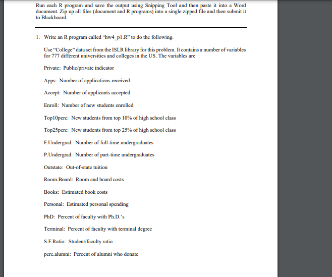
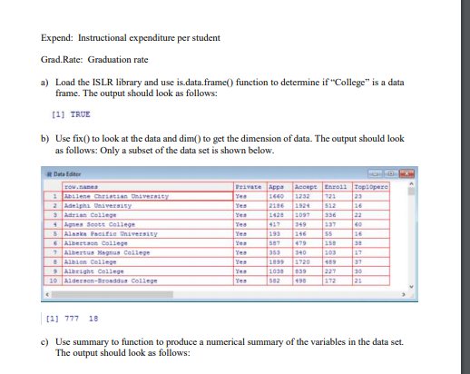
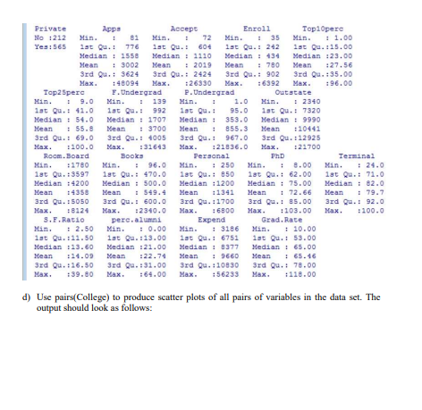
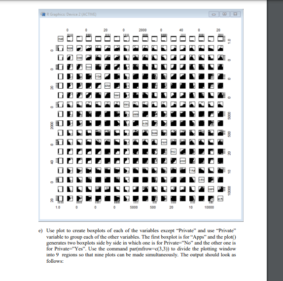
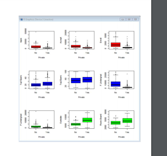
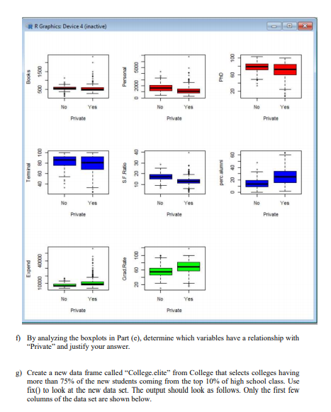
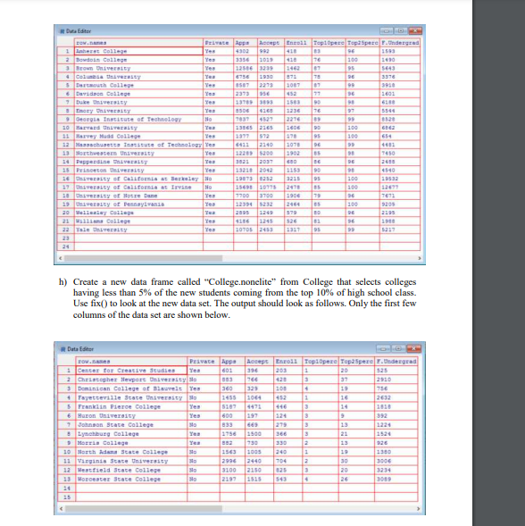
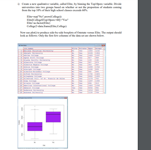
Topic: Machine Learning Run cach R program and save the output using Snipping Tool and then paste it into a Word document. Zip up all

Topic: Machine Learning

image text in transcribedimage text in transcribedimage text in transcribedimage text in transcribedimage text in transcribedimage text in transcribedimage text in transcribedimage text in transcribed

Run cach R program and save the output using Snipping Tool and then paste it into a Word document. Zip up all files (document and R programs) into a single zipped file and then submit it to Blackboard. 1. Write an R program called "hw4_p1.R to do the following. Use "College" data set from the ISLR library for this problem. It contains a number of variables for 777 different universities and colleges in the US. The variables are Private: Public/private indicator Apps: Number of applications received Accept: Number of applicants accepted Enroll: Number of new students enrolled Top10perc: New students from top 10% of high school class Top25perc: New students from top 25% of high school class F.Undergrad: Number of full-time undergraduates P.Undergrad: Number of part-time undergraduates Outstate: Out-of-state tuition Room.Board: Room and board costs Books: Estimated book costs Personal: Estimated personal spending PhD: Percent of faculty with Ph.D.'s Terminal: Percent of faculty with terminal degree S.F.Ratio: Student/faculty ratio perc.alumni: Percent of alumni who donate Expend: Instructional expenditure per student Grad. Rate: Graduation rate a) Load the ISLR library and use is.data.frame() function to determine if "College" is a data frame. The output should look as follows: [1] TRUE b) Use fix() to look at the data and dim() to get the dimension of data. The output should look as follows: Only a subset of the data set is shown below. Date Editor Date Appa Yes 2106 1420 Yes 1 Alene Christian LVTALE 2 Adelphi University 3 Adrian College 4 Agnes Scott College 5 Alaska Pacific University 6 Albertson College 7 Albertus Magnus College Albion College Albright College 10 Alderson-Broaddus College Accepe Caroll Teplopere 123 23 512 1097 336 22 137 116 55 16 679 153 30 340 1720 189 37 839 30 498 172 21 193 582 353 1899 1038 502 Yes Yes 103 Yes Yes [2] 777 18 c) Use summary to function to produce a numerical summary of the variables in the data set. The output should look as follows: Private Apps Accept Enroll Top10perc NO :212 Min. 81 Min. : 72 Min. 35 Min. 11.00 Yes: 565 1st Qu.: 776 1st Qu.: 604 1st Qu.: 242 1st Qu. 115.00 Median : 1558 Median : 1110 Median : 434 Median :23.00 Mean 3002 Mean 2019 Mean: 780 Mean 127.56 3rd Qu. : 3624 3rd Qu.: 2424 3rd Qu.: 902 3rd Qu. 135.00 Max. 48094 Max. : 26330 Max. : 6392 Max. :96.00 Top25perc F.Undergrad P. Undergrad Outstate Min. 139 Min. 1.0Min. 2340 lat Qu. 11.0 lat Qu.: 992 95.0 1st Qu.: 7320 Median : 54.0 Median : 1707 Median: 353.0 Median 9990 Mean 55.8 Mean : 3700 Mean : 855.3 Mean 10441 3rd Qu.: 69.0 3rd Qu.: 4005 3rd Qu.: 967.0 3rd Qu. 112925 Max. 1100.0 Max. +31643 Max. 121836.0 Max. 21700 Room. Board Books Personal PhD Terminal : 1780 Min. 96.0 Min. 250 Min. 8.00 Min. : 24.0 1st Qu. : 3597 1st Qu.: 470.0 1st Qu. 1 850 180 Qu.: 62.00 1st Qu. : 71.0 Median : 4200 Median : 500.0 Median :1200 Median: 75.00 Median: 82.0 Mean 14358 Mean 549.4 Mean 11341 Mean : 72.66 Mean 79.7 3rd Qu.:5050 3rd Qu.: 600.0 3rd Qu. :1700 3rd Qu.: 85.00 3rd Qu.: 92.0 Max. :8124 Max. :2340.0 Max. : 6800 Max. :103.00 Max. :100.0 3. F. Ratio pere. alumni Expend Grad. Rate Min. 2.50 Min. : 0.00 Min. 3186 Min. 10.00 1st Qu. 11.50 1st Qu. 13.00 1st Qu.: 6751 1st Qu. : 53.00 Median :13.60 Median :21.00 Median : 8377 Median : 65.00 Mean 14.09 Mean :22.74 Mean : 9660 Mean : 65.46 3rd Qu. 116.50 3rd Qu. 131.00 3rd Qu. :10830 3rd Qu.: 78.00 Max. +39.80 Max. :64.00 Max. :56233 Max. :118.00 d) Use pairs(College) to produce scatter plots of all pairs of variables in the data set. The output should look as follows: RR Graphic Device 2 (ACTIVE) 2000 LE LE 1 U DO DOS 1 . 0 0005 000 20 10 10000 10 5000 500 10000 c) Use plot to create boxplots of each of the variables except "Private" and use "Private" variable to group each of the other variables. The first boxplot is for "Apps and the plot() generates two boxplots side by side in which one is for Private="No" and the other one is for Private="Yes". Use the command par(mfrow=c(3,3)) to divide the plotting window into 9 regions so that nine plots can be made simultaneously. The output should look as follows: RR Graphics: Device 3 (inactive) D 23 50000 000SC Apps 20000 --+ 10000 Enrol 0 2000 5000 0 0 Yes No Yes NO Yes Private Private 100 Top1Operc Top 25perc 60 0 10000 25000 20 No Yes No Yes No Yes Private Private Private PUndergrad 10000 20000 Outstate 15000 Room Board 2000 5000 8000 5000 0 No Yes No Yes No Yes Private Private Private RR Graphics: Device 4 (inactive) 100 Books -+ Personal 0 2000 5000 PNO 500 Yes No No Yes Private Private Private Terminal 40 60 80 100 SF Ratio 10 20 30 40 LLL per un 0 20 40 60 No Yes No Yes No Yes Private Expend 10000 40000 Grad Rate 20 60 100 No Yes No Yes Private Private f) By analyzing the boxplots in Part (e), determine which variables have a relationship with "Private" and justify your answer. g) Create a new data frame called "College.elite" from College that selects colleges having more than 75% of the new students coming from the top 10% of high school class. Use fix() to look at the new data set. The output should look as follows. Only the first few columns of the data set are shown below. Duta Editor Recep Enroll Tepl Opere Toppere Undergrad 1593 3356 101) 10 76 100 100 1463 95 6756 1990 17 3376 2273 99 2373 95 96 1601 13789383 1236 76 13165 2165 100E 1 hrs College Yes 2 Dowdon College Yes Brown Diversity Yes 4 Columna very 5 Douth College Yer 6 Davidson College Diversity Yes Boty Chi 9 Dorota Institute of Technology No 10 Harvard University 11 Barvey Mud College Yes 12 Machusetts Institute of Technology Yes 13 Borchester Unit Yes 14 Pepperdine nivel Yes Princeton Yes 16 Dverity of California at Berkeley NO 17 University of California at Irvine No 30 DEVET O Morre Dame 19 Diversity of Pennsylvania Yes 20 Wellesley College 2140 12289 5200 2092 13211 2012 1078 1902 60 1153 95 96 85 DE 90 90 DE 93 7450 240 4510 126 15693 10175 7700 2018 1906 85 79 100 06 9205 579 ED BE 116 1215 30705243 22 Yale y Yos 95 24 h) Create a new data frame called "College.nonelite from College that selects colleges having less than 5% of the new students coming from the top 10% of high school class. Use fix() to look at the new data set. The output should look as follows. Only the first few columns of the data set are shown below. #Dute Editor LOW.SE Private Appa 1 Center for Creative Studies Yes 601 2 Christopher Newport University 383 3 Dominican College of Surelt Yes 360 Tayetteville State University 5 Franklin Pierce College Yes 6 Huron University Yes 600 Johnson State College No Lynchburg College Yes 1750 Mornia College 10 North Am State College 1563 Virginia State University Na 2996 12 Westfield State College 3100 13 Worcester State College Slo 2197 Acceps Enroll Topi Opere Top25pere Undergrad 394 1 20 525 760 37 2910 4 19 1064 1 16 2632 3 124 3 669 279 3 13 1500 360 3 21 730 13 126 1005 240 1 19 1380 2440 704 2 30 3006 2150 3 20 3234 543 1 15 60)="Yes" Elite=as.factor(Elite) College2=data.frame(Elite, College) Now use plot() to produce side-by-side boxplots of Outstate versus Elite. The output should look as follows: Only the first few columns of the data set are shown below. Elite Private Apps Accept NO Yes Mo Yes 2186 1924 349 146 Yes No No No Mo Yes Yes Ow.am 1 Abilene Chan University 2 Adelphi University 3 Adrian College 4 Agnes Scott College 5 Alaska Pacific University 6 Albertson College 7 Albertus Magnus college Albion College 9 Albright college 10 Alderson-Broaddus College 11 Alfred University 12 Allegheny College 13 Allentown Coll, of st. Francis de Sales 14 Ans college 15 Alverno College 16 American International college 17 best college 18 Anderson University 19 Andrews University 193 587 353 1899 1036 592 173 2652 1179 1267 Yes NO Na No No No IND NO Yes 1720 839 498 1425 1900 780 10 313 1093 Yes Yes Yes 120 1216 1130 704 1 Run cach R program and save the output using Snipping Tool and then paste it into a Word document. Zip up all files (document and R programs) into a single zipped file and then submit it to Blackboard. 1. Write an R program called "hw4_p1.R to do the following. Use "College" data set from the ISLR library for this problem. It contains a number of variables for 777 different universities and colleges in the US. The variables are Private: Public/private indicator Apps: Number of applications received Accept: Number of applicants accepted Enroll: Number of new students enrolled Top10perc: New students from top 10% of high school class Top25perc: New students from top 25% of high school class F.Undergrad: Number of full-time undergraduates P.Undergrad: Number of part-time undergraduates Outstate: Out-of-state tuition Room.Board: Room and board costs Books: Estimated book costs Personal: Estimated personal spending PhD: Percent of faculty with Ph.D.'s Terminal: Percent of faculty with terminal degree S.F.Ratio: Student/faculty ratio perc.alumni: Percent of alumni who donate Expend: Instructional expenditure per student Grad. Rate: Graduation rate a) Load the ISLR library and use is.data.frame() function to determine if "College" is a data frame. The output should look as follows: [1] TRUE b) Use fix() to look at the data and dim() to get the dimension of data. The output should look as follows: Only a subset of the data set is shown below. Date Editor Date Appa Yes 2106 1420 Yes 1 Alene Christian LVTALE 2 Adelphi University 3 Adrian College 4 Agnes Scott College 5 Alaska Pacific University 6 Albertson College 7 Albertus Magnus College Albion College Albright College 10 Alderson-Broaddus College Accepe Caroll Teplopere 123 23 512 1097 336 22 137 116 55 16 679 153 30 340 1720 189 37 839 30 498 172 21 193 582 353 1899 1038 502 Yes Yes 103 Yes Yes [2] 777 18 c) Use summary to function to produce a numerical summary of the variables in the data set. The output should look as follows: Private Apps Accept Enroll Top10perc NO :212 Min. 81 Min. : 72 Min. 35 Min. 11.00 Yes: 565 1st Qu.: 776 1st Qu.: 604 1st Qu.: 242 1st Qu. 115.00 Median : 1558 Median : 1110 Median : 434 Median :23.00 Mean 3002 Mean 2019 Mean: 780 Mean 127.56 3rd Qu. : 3624 3rd Qu.: 2424 3rd Qu.: 902 3rd Qu. 135.00 Max. 48094 Max. : 26330 Max. : 6392 Max. :96.00 Top25perc F.Undergrad P. Undergrad Outstate Min. 139 Min. 1.0Min. 2340 lat Qu. 11.0 lat Qu.: 992 95.0 1st Qu.: 7320 Median : 54.0 Median : 1707 Median: 353.0 Median 9990 Mean 55.8 Mean : 3700 Mean : 855.3 Mean 10441 3rd Qu.: 69.0 3rd Qu.: 4005 3rd Qu.: 967.0 3rd Qu. 112925 Max. 1100.0 Max. +31643 Max. 121836.0 Max. 21700 Room. Board Books Personal PhD Terminal : 1780 Min. 96.0 Min. 250 Min. 8.00 Min. : 24.0 1st Qu. : 3597 1st Qu.: 470.0 1st Qu. 1 850 180 Qu.: 62.00 1st Qu. : 71.0 Median : 4200 Median : 500.0 Median :1200 Median: 75.00 Median: 82.0 Mean 14358 Mean 549.4 Mean 11341 Mean : 72.66 Mean 79.7 3rd Qu.:5050 3rd Qu.: 600.0 3rd Qu. :1700 3rd Qu.: 85.00 3rd Qu.: 92.0 Max. :8124 Max. :2340.0 Max. : 6800 Max. :103.00 Max. :100.0 3. F. Ratio pere. alumni Expend Grad. Rate Min. 2.50 Min. : 0.00 Min. 3186 Min. 10.00 1st Qu. 11.50 1st Qu. 13.00 1st Qu.: 6751 1st Qu. : 53.00 Median :13.60 Median :21.00 Median : 8377 Median : 65.00 Mean 14.09 Mean :22.74 Mean : 9660 Mean : 65.46 3rd Qu. 116.50 3rd Qu. 131.00 3rd Qu. :10830 3rd Qu.: 78.00 Max. +39.80 Max. :64.00 Max. :56233 Max. :118.00 d) Use pairs(College) to produce scatter plots of all pairs of variables in the data set. The output should look as follows: RR Graphic Device 2 (ACTIVE) 2000 LE LE 1 U DO DOS 1 . 0 0005 000 20 10 10000 10 5000 500 10000 c) Use plot to create boxplots of each of the variables except "Private" and use "Private" variable to group each of the other variables. The first boxplot is for "Apps and the plot() generates two boxplots side by side in which one is for Private="No" and the other one is for Private="Yes". Use the command par(mfrow=c(3,3)) to divide the plotting window into 9 regions so that nine plots can be made simultaneously. The output should look as follows: RR Graphics: Device 3 (inactive) D 23 50000 000SC Apps 20000 --+ 10000 Enrol 0 2000 5000 0 0 Yes No Yes NO Yes Private Private 100 Top1Operc Top 25perc 60 0 10000 25000 20 No Yes No Yes No Yes Private Private Private PUndergrad 10000 20000 Outstate 15000 Room Board 2000 5000 8000 5000 0 No Yes No Yes No Yes Private Private Private RR Graphics: Device 4 (inactive) 100 Books -+ Personal 0 2000 5000 PNO 500 Yes No No Yes Private Private Private Terminal 40 60 80 100 SF Ratio 10 20 30 40 LLL per un 0 20 40 60 No Yes No Yes No Yes Private Expend 10000 40000 Grad Rate 20 60 100 No Yes No Yes Private Private f) By analyzing the boxplots in Part (e), determine which variables have a relationship with "Private" and justify your answer. g) Create a new data frame called "College.elite" from College that selects colleges having more than 75% of the new students coming from the top 10% of high school class. Use fix() to look at the new data set. The output should look as follows. Only the first few columns of the data set are shown below. Duta Editor Recep Enroll Tepl Opere Toppere Undergrad 1593 3356 101) 10 76 100 100 1463 95 6756 1990 17 3376 2273 99 2373 95 96 1601 13789383 1236 76 13165 2165 100E 1 hrs College Yes 2 Dowdon College Yes Brown Diversity Yes 4 Columna very 5 Douth College Yer 6 Davidson College Diversity Yes Boty Chi 9 Dorota Institute of Technology No 10 Harvard University 11 Barvey Mud College Yes 12 Machusetts Institute of Technology Yes 13 Borchester Unit Yes 14 Pepperdine nivel Yes Princeton Yes 16 Dverity of California at Berkeley NO 17 University of California at Irvine No 30 DEVET O Morre Dame 19 Diversity of Pennsylvania Yes 20 Wellesley College 2140 12289 5200 2092 13211 2012 1078 1902 60 1153 95 96 85 DE 90 90 DE 93 7450 240 4510 126 15693 10175 7700 2018 1906 85 79 100 06 9205 579 ED BE 116 1215 30705243 22 Yale y Yos 95 24 h) Create a new data frame called "College.nonelite from College that selects colleges having less than 5% of the new students coming from the top 10% of high school class. Use fix() to look at the new data set. The output should look as follows. Only the first few columns of the data set are shown below. #Dute Editor LOW.SE Private Appa 1 Center for Creative Studies Yes 601 2 Christopher Newport University 383 3 Dominican College of Surelt Yes 360 Tayetteville State University 5 Franklin Pierce College Yes 6 Huron University Yes 600 Johnson State College No Lynchburg College Yes 1750 Mornia College 10 North Am State College 1563 Virginia State University Na 2996 12 Westfield State College 3100 13 Worcester State College Slo 2197 Acceps Enroll Topi Opere Top25pere Undergrad 394 1 20 525 760 37 2910 4 19 1064 1 16 2632 3 124 3 669 279 3 13 1500 360 3 21 730 13 126 1005 240 1 19 1380 2440 704 2 30 3006 2150 3 20 3234 543 1 15 60)="Yes" Elite=as.factor(Elite) College2=data.frame(Elite, College) Now use plot() to produce side-by-side boxplots of Outstate versus Elite. The output should look as follows: Only the first few columns of the data set are shown below. Elite Private Apps Accept NO Yes Mo Yes 2186 1924 349 146 Yes No No No Mo Yes Yes Ow.am 1 Abilene Chan University 2 Adelphi University 3 Adrian College 4 Agnes Scott College 5 Alaska Pacific University 6 Albertson College 7 Albertus Magnus college Albion College 9 Albright college 10 Alderson-Broaddus College 11 Alfred University 12 Allegheny College 13 Allentown Coll, of st. Francis de Sales 14 Ans college 15 Alverno College 16 American International college 17 best college 18 Anderson University 19 Andrews University 193 587 353 1899 1036 592 173 2652 1179 1267 Yes NO Na No No No IND NO Yes 1720 839 498 1425 1900 780 10 313 1093 Yes Yes Yes 120 1216 1130 704 1

Step by Step Solution

There are 3 Steps involved in it

Step: 1

blur-text-image

Get Instant Access to Expert-Tailored Solutions

See step-by-step solutions with expert insights and AI powered tools for academic success

Step: 2

blur-text-image

Step: 3

blur-text-image

Ace Your Homework with AI

Get the answers you need in no time with our AI-driven, step-by-step assistance

Get Started

Recommended Textbook for

Big Data With Hadoop MapReduce A Classroom Approach

Authors: Rathinaraja Jeyaraj ,Ganeshkumar Pugalendhi ,Anand Paul

1st Edition

1774634848, 978-1774634844

More Books

Students also viewed these Databases questions

Question

Describe interpersonal skills related to social networking.

Answered: 1 week ago

Question

1. In what ways has flexible working revolutionised employment?

Answered: 1 week ago