type	Q1	Q2	Q3	Q4	Total
mini	2,290	2,297	2,298	2,289	9,174
voice activated	1,509	1,509	1,514	1,511	6,043
water proof	1,517	1,520	1,524	1,528	6,089
total	5,316	5,326	5,336	5,328	21,309

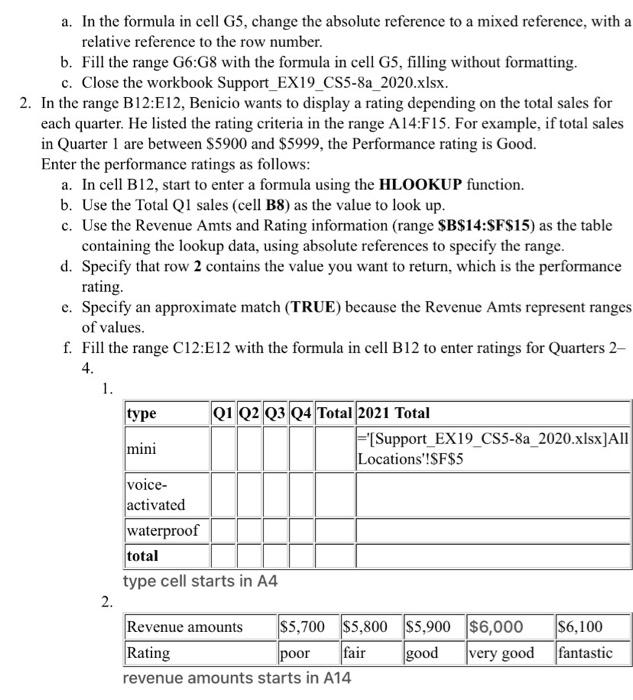
This is the Table being referenced in G5.

From workheet Support_EX19_CS5-8a_2020.xlsx.

This tabel starts in A3

For clarification-

first table is the table being worked on.

second table is referece table used for Questions in number 2

3rd table is other document table used for the first a,b,c questions

a. In the formula in cell G5, change the absolute reference to a mixed reference, with a relative reference to the row number. b. Fill the range G6:08 with the formula in cell G5, filling without formatting. c. Close the workbook Support_EX19_CS5-8a_2020.xlsx. 2. In the range B12:E12, Benicio wants to display a rating depending on the total sales for each quarter. He listed the rating criteria in the range A14:F15. For example, if total sales in Quarter 1 are between $5900 and $5999, the Performance rating is Good. Enter the performance ratings as follows: a. In cell B12, start to enter a formula using the HLOOKUP function. b. Use the Total Q1 sales (cell B8) as the value to look up. c. Use the Revenue Amts and Rating information (range $B$14:$F$15) as the table containing the lookup data, using absolute references to specify the range. d. Specify that row 2 contains the value you want to return, which is the performance rating e. Specify an approximate match (TRUE) because the Revenue Amts represent ranges of values. f. Fill the range C12:E12 with the formula in cell B12 to enter ratings for Quarters 2- 4. 1. Q1 Q2 Q3 Q4 Total 2021 Total mini F'[Support_EX19_CS5-8a_2020.xlsx]All Locations'!$F$5 voice- activated waterproof total type cell starts in A4 2. Revenue amounts $5,700 $5,800 $5,900 $6,000 $6,100 poor fair good very good fantastic revenue amounts starts in A14 type Rating a. In the formula in cell G5, change the absolute reference to a mixed reference, with a relative reference to the row number. b. Fill the range G6:08 with the formula in cell G5, filling without formatting. c. Close the workbook Support_EX19_CS5-8a_2020.xlsx. 2. In the range B12:E12, Benicio wants to display a rating depending on the total sales for each quarter. He listed the rating criteria in the range A14:F15. For example, if total sales in Quarter 1 are between $5900 and $5999, the Performance rating is Good. Enter the performance ratings as follows: a. In cell B12, start to enter a formula using the HLOOKUP function. b. Use the Total Q1 sales (cell B8) as the value to look up. c. Use the Revenue Amts and Rating information (range $B$14:$F$15) as the table containing the lookup data, using absolute references to specify the range. d. Specify that row 2 contains the value you want to return, which is the performance rating e. Specify an approximate match (TRUE) because the Revenue Amts represent ranges of values. f. Fill the range C12:E12 with the formula in cell B12 to enter ratings for Quarters 2- 4. 1. Q1 Q2 Q3 Q4 Total 2021 Total mini F'[Support_EX19_CS5-8a_2020.xlsx]All Locations'!$F$5 voice- activated waterproof total type cell starts in A4 2. Revenue amounts $5,700 $5,800 $5,900 $6,000 $6,100 poor fair good very good fantastic revenue amounts starts in A14 type Rating