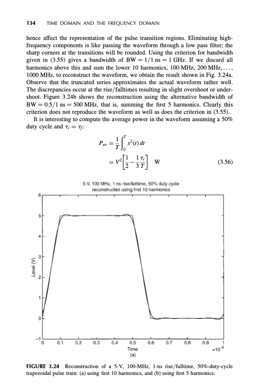
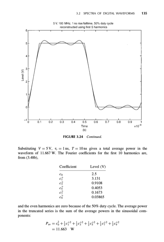
Understanding the Fourier series (40 points) First, review section 3.2.2.2 of your textbook. Then, to understand the implications of the number of harmonics used to reconstruct a signal, consider the following case. Assume you have a trapezoidal waveform characterized by the fundamental frequency fo = 4 GHz, 50% duty cycle, Tp = Tf T/50, where t = = T/2 and T is the period. Write a Matlab program that computes a plot with the following 3 waveforms: = T 1. The exact waveform. 2. The waveform reconstructed using a number N of harmonics, where N is the smallest number for which Nifo > 1/(at) 3. The waveform reconstructed using a number N2 of harmonics, where N2 is the smallest number for which N2 fo> 1/(TT) Based upon the results of your reconstruction, would you approximate the maximum frequency of the ap- proximated trapezoidal waveform with (1) Nifo or (2) N2fo ? 3.2.2.2 Bandwidth of Digital Waveforms It is clear from the Fourier series that in order to completely reconstruct a time-domain waveform from its spectral content, we must sum an infinite number of harmonics. Clearly, this is not practical. If we continue to add spectral harmonics to the sum, the resulting time-domain waveform gets closer to the actual complete waveform. (There is a phenomenon known as Gibb's phenomenon, which occurs at points in a waveform that are discon- tinuous such as the rising and falling edges of a square wave. The ideal square wave has zero rise/falltimes, and continually adding harmonics will not result in conver- gence to ideal waveforms at these abrupt discontinuities. The important question is how many of the harmonics must we add in order to reconstruct a waveform that is in some fashion a reasonable approximation to the actual time-domain waveform? A fundamental property of the Fourier series and the way the coefficients are com- puted as in (3.12) is that this choice of the coefficients will minimize the integral squared error (ISE) between the actual waveform and the approximate one using 3.2 SPECTRA OF DIGITAL WAVEFORMS 133 the first N coefficients (2]. The integral squared error is +T ISE = L" [x(1) - 200 dt where the finite N-term expansion is denoted as (t) = c(1) NEM The expansion coefficients are orthogonal functions by choice, and orthogonal basis functions have the important property of minimizing the approximation error when we truncate the expansion, that is, use a finite number of expansion terms or spectral components. The ISE reflects the fact that t "positive error" at a particular timer, li.e., x(0) (0)] is as bad as a "negative error" [i.e., 2(1) > x(0)). But this does not really give a measure of how close the approximation is to the actual function at individual points; that is, we might have very close agreement at almost every time- point but have an extraordinarily large error at a few points and yet the ISE may look "good. Perhaps the best we can do is to include the harmonics up to a point, truncate the sum, and how well the reconstructed function matches the actual waveform. If we look at the spectral bound model of a digital (trapezoidal) waveform shown in Fig. 3.19, we see that above the second breakpoint, 1/TTT,, the harmonics drop off at a rate of -40 dB/decade. Hence if we remove spectral components above this, the time-domain waveform would probably not be sufficiently distorted" from the actual waveform. To be conservative we might choose a point, say, 3 times this second breakpoint or 3/TT. But this is approximately 1/Tr. Hence we might choose the "bandwidth" of this digital clock signal BW = Hz (3.55) For example, a signal having a rise/falltime of 1 ns would have, by this criterion, a bandwidth of 1 GHz. Others have chosen a criterion for bandwidth as 0.5/Tr. (See Chapter 1 Ref. 14.) This criterion is not meant to be a hard criterion but is to be used only as a guide to estimate how much of the spectrum is needed to produce an "accurate" reproduction of the time-domain waveform. It is interesting to observe from (3.48) that the first null in the true spectrum occurs at f = 1/T, (substitute nit,/T TT, in the second sinx/x term). In order to investigate this we show, in Fig. 3.24a, a comparison of reconstructing a trapezoidal waveform using only the spectral components up to a frequency of 1/T, for a 100-MHz, 50%-duty-cycle, 5-V trapezoidal (clock) waveform having 1 ns rise/falltimes. Typically the lower frequencies of the spectrum affect the level of the pulse, while the higher frequencies affect the sharp edges. So eliminating the high-frequency components of the spectrum tends to roll off the sharp edges and 134 TIME DOMAIN AND THE FREQUENCY DOMAIN hence affect the representation of the pulse transition regions. Eliminating high- frequency components is like passing the waveform through a low pass filter; the sharp corners at the transitions will be rounded. Using the criterion for bandwidth given in (3.55) gives a bandwidth of BW = 1/1 ns = 1 GHz. If we discard all harmonics above this and sum the lower 10 harmonics, 100 MHz, 200 MHz, ..., 1000 MHz, to reconstruct the waveform, we obtain the result shown in Fig. 3.24a. Observe that the truncated series approximates the actual waveform rather well. The discrepancies occur at the rise/falltimes resulting in slight overshoot or under- shoot. Figure 3.24b shows the reconstruction using the alternative bandwidth of BW = 0.5/1 ns = 500 MHz, that is, summing the first 5 harmonics. Clearly this criterion does not reproduce the waveform as well as does the criterion in (3.55). It is interesting to compute the average power in the waveform assuming a 50% duty cycle and T, = Tj: + () di V[1 W 37 (3.56) 5 V, 100 MHz, 1 ns rise/falltime, 50% duty cyde reconstructed using first 10 harmonics BH Level (V) 21 1 0 0 0.1 02 0.3 0.4 0.6 0.7 0.8 0.9 0.5 Time (a) 1 x10 -8 FIGURE 3.24 Reconstruction of a 5-V, 100-MHz, 1-ns rise/falltime, 50%-duty-cycle trapezoidal pulse train: (a) using first 10 harmonics, and (b) using first 5 harmonics. 3.2 SPECTRA OF DIGITAL WAVEFORMS 135 5V, 100 MHz, 1ns rise/tolltime, 50% duly cycle reconstructed using first 5 harmonios 31 Level() 2H 0.1 0.2 0.4 0.6 0.7 0.8 0.9 1 0.5 Time (b) *10 FIGURE 3.24 Continued. Substituting V = 5V, 1, = 1ns, T = 10 ns gives a total average power in the waveform of 11.667 W. The Fourier coefficients for the first 10 harmonics are, from (3.48b). Coefficient Level (V) 2.5 ct 3.131 0.9108 0.4053 0.1673 0.03865 and the even harmonies are zero because of the 50% duty cycle. The average power in the truncated series is the sum of the average powers in the sinusoidal com- ponents: Par = c +302+0+2 + $c$2 + c+2 +3442 = 11.663 W 136 TIME DOMAIN AND THE FREQUENCY DOMAIN Hence the average power in the truncated series is 99.97% of the total average power in the periodic waveform. In the alternative criterion of bandwidth, BW = 0.5/Tr. the average power in this truncated sum consisting of 5 harmonics is 11.648 W or 99.84% of the total. In both cases, the truncated series contains virtually all the average power in the complete waveform, so that looking at the average power contained in the truncated series is not a satisfactory criterion for judging its ability to reproduce the waveform and hence the bandwidth. In fact, for this wave- form, 96% of the total average power of the waveform is contained in the de term and the first harmonic. Review Exercise 3.3 For a trapezoidal waveform having equal rise and falltimes, determine how much the bound is down at f = 1/T, from the level at the second breakpoint of 1/ TTT Answer: 19.89 dB. Understanding the Fourier series (40 points) First, review section 3.2.2.2 of your textbook. Then, to understand the implications of the number of harmonics used to reconstruct a signal, consider the following case. Assume you have a trapezoidal waveform characterized by the fundamental frequency fo = 4 GHz, 50% duty cycle, Tp = Tf T/50, where t = = T/2 and T is the period. Write a Matlab program that computes a plot with the following 3 waveforms: = T 1. The exact waveform. 2. The waveform reconstructed using a number N of harmonics, where N is the smallest number for which Nifo > 1/(at) 3. The waveform reconstructed using a number N2 of harmonics, where N2 is the smallest number for which N2 fo> 1/(TT) Based upon the results of your reconstruction, would you approximate the maximum frequency of the ap- proximated trapezoidal waveform with (1) Nifo or (2) N2fo ? 3.2.2.2 Bandwidth of Digital Waveforms It is clear from the Fourier series that in order to completely reconstruct a time-domain waveform from its spectral content, we must sum an infinite number of harmonics. Clearly, this is not practical. If we continue to add spectral harmonics to the sum, the resulting time-domain waveform gets closer to the actual complete waveform. (There is a phenomenon known as Gibb's phenomenon, which occurs at points in a waveform that are discon- tinuous such as the rising and falling edges of a square wave. The ideal square wave has zero rise/falltimes, and continually adding harmonics will not result in conver- gence to ideal waveforms at these abrupt discontinuities. The important question is how many of the harmonics must we add in order to reconstruct a waveform that is in some fashion a reasonable approximation to the actual time-domain waveform? A fundamental property of the Fourier series and the way the coefficients are com- puted as in (3.12) is that this choice of the coefficients will minimize the integral squared error (ISE) between the actual waveform and the approximate one using 3.2 SPECTRA OF DIGITAL WAVEFORMS 133 the first N coefficients (2]. The integral squared error is +T ISE = L" [x(1) - 200 dt where the finite N-term expansion is denoted as (t) = c(1) NEM The expansion coefficients are orthogonal functions by choice, and orthogonal basis functions have the important property of minimizing the approximation error when we truncate the expansion, that is, use a finite number of expansion terms or spectral components. The ISE reflects the fact that t "positive error" at a particular timer, li.e., x(0) (0)] is as bad as a "negative error" [i.e., 2(1) > x(0)). But this does not really give a measure of how close the approximation is to the actual function at individual points; that is, we might have very close agreement at almost every time- point but have an extraordinarily large error at a few points and yet the ISE may look "good. Perhaps the best we can do is to include the harmonics up to a point, truncate the sum, and how well the reconstructed function matches the actual waveform. If we look at the spectral bound model of a digital (trapezoidal) waveform shown in Fig. 3.19, we see that above the second breakpoint, 1/TTT,, the harmonics drop off at a rate of -40 dB/decade. Hence if we remove spectral components above this, the time-domain waveform would probably not be sufficiently distorted" from the actual waveform. To be conservative we might choose a point, say, 3 times this second breakpoint or 3/TT. But this is approximately 1/Tr. Hence we might choose the "bandwidth" of this digital clock signal BW = Hz (3.55) For example, a signal having a rise/falltime of 1 ns would have, by this criterion, a bandwidth of 1 GHz. Others have chosen a criterion for bandwidth as 0.5/Tr. (See Chapter 1 Ref. 14.) This criterion is not meant to be a hard criterion but is to be used only as a guide to estimate how much of the spectrum is needed to produce an "accurate" reproduction of the time-domain waveform. It is interesting to observe from (3.48) that the first null in the true spectrum occurs at f = 1/T, (substitute nit,/T TT, in the second sinx/x term). In order to investigate this we show, in Fig. 3.24a, a comparison of reconstructing a trapezoidal waveform using only the spectral components up to a frequency of 1/T, for a 100-MHz, 50%-duty-cycle, 5-V trapezoidal (clock) waveform having 1 ns rise/falltimes. Typically the lower frequencies of the spectrum affect the level of the pulse, while the higher frequencies affect the sharp edges. So eliminating the high-frequency components of the spectrum tends to roll off the sharp edges and 134 TIME DOMAIN AND THE FREQUENCY DOMAIN hence affect the representation of the pulse transition regions. Eliminating high- frequency components is like passing the waveform through a low pass filter; the sharp corners at the transitions will be rounded. Using the criterion for bandwidth given in (3.55) gives a bandwidth of BW = 1/1 ns = 1 GHz. If we discard all harmonics above this and sum the lower 10 harmonics, 100 MHz, 200 MHz, ..., 1000 MHz, to reconstruct the waveform, we obtain the result shown in Fig. 3.24a. Observe that the truncated series approximates the actual waveform rather well. The discrepancies occur at the rise/falltimes resulting in slight overshoot or under- shoot. Figure 3.24b shows the reconstruction using the alternative bandwidth of BW = 0.5/1 ns = 500 MHz, that is, summing the first 5 harmonics. Clearly this criterion does not reproduce the waveform as well as does the criterion in (3.55). It is interesting to compute the average power in the waveform assuming a 50% duty cycle and T, = Tj: + () di V[1 W 37 (3.56) 5 V, 100 MHz, 1 ns rise/falltime, 50% duty cyde reconstructed using first 10 harmonics BH Level (V) 21 1 0 0 0.1 02 0.3 0.4 0.6 0.7 0.8 0.9 0.5 Time (a) 1 x10 -8 FIGURE 3.24 Reconstruction of a 5-V, 100-MHz, 1-ns rise/falltime, 50%-duty-cycle trapezoidal pulse train: (a) using first 10 harmonics, and (b) using first 5 harmonics. 3.2 SPECTRA OF DIGITAL WAVEFORMS 135 5V, 100 MHz, 1ns rise/tolltime, 50% duly cycle reconstructed using first 5 harmonios 31 Level() 2H 0.1 0.2 0.4 0.6 0.7 0.8 0.9 1 0.5 Time (b) *10 FIGURE 3.24 Continued. Substituting V = 5V, 1, = 1ns, T = 10 ns gives a total average power in the waveform of 11.667 W. The Fourier coefficients for the first 10 harmonics are, from (3.48b). Coefficient Level (V) 2.5 ct 3.131 0.9108 0.4053 0.1673 0.03865 and the even harmonies are zero because of the 50% duty cycle. The average power in the truncated series is the sum of the average powers in the sinusoidal com- ponents: Par = c +302+0+2 + $c$2 + c+2 +3442 = 11.663 W 136 TIME DOMAIN AND THE FREQUENCY DOMAIN Hence the average power in the truncated series is 99.97% of the total average power in the periodic waveform. In the alternative criterion of bandwidth, BW = 0.5/Tr. the average power in this truncated sum consisting of 5 harmonics is 11.648 W or 99.84% of the total. In both cases, the truncated series contains virtually all the average power in the complete waveform, so that looking at the average power contained in the truncated series is not a satisfactory criterion for judging its ability to reproduce the waveform and hence the bandwidth. In fact, for this wave- form, 96% of the total average power of the waveform is contained in the de term and the first harmonic. Review Exercise 3.3 For a trapezoidal waveform having equal rise and falltimes, determine how much the bound is down at f = 1/T, from the level at the second breakpoint of 1/ TTT Answer: 19.89 dB