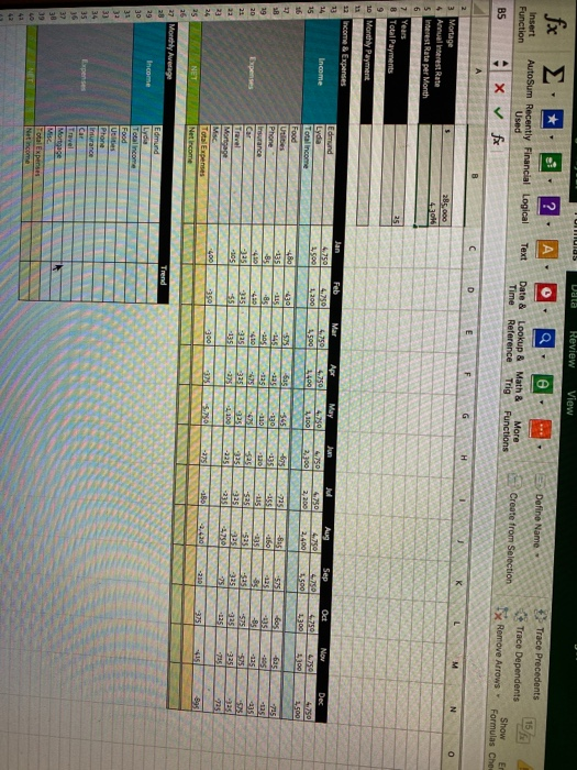
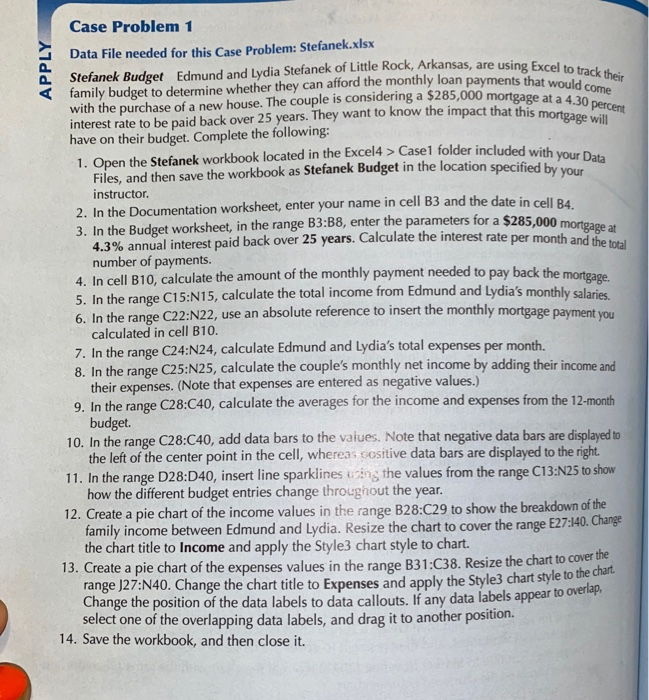
UNTUIUS Data Review View 0 Define Name Insert Function ? AutoSum Recently Financial Logical Used Xfx 15 Text Date & Lookup & Math & Time Reference Trig More * Trace Precedents Trace Dependents 1 Remove Arrows Functions Create from Selection BS Show Er Formulas Che D E F G H M N Mortage Annual interest Rate Interest Rate per Month 6 285,000 432016 7 Years 8 Total Payments 251 10 Monthly Payment 12 Income & Expenses Mar Edmund Jan 5.750 Feb 4.750 Apr 4.750 May Jun Income Jul 6.750 2,200 5.750 1,500 1,200 Aug 4.750 2,400 2.100 Sep 4.750 3.500 Oct 4.750 1300 2.300 Nov 4.750 1300 Dec 4.750 1.500 -575 Total income Food Utilities Phone Insurance Car -480 -135 -85 -410 SR 19 20 -625 -675 -135 130 725 -115 -8 -450 05 -135-130 -725 -155 -115 5251 -835 160 -135 -575 25 8 tes 335 -B Expenses -135 21 23 23 325 3229 -135 -105 Mortage 1200 -335 -335 2775 3325 135 325 75 400 2350 300 5. Total Expenses Net income -225 -130 -210 15 895 24 25 NET 26 27 Monthly Average Trend Edmund Income 29 30 31 22 33 34 35 16 32 Total income Food Ulties Phone Insurance Car Mortgage 39 LO 42 42 Total Expenses Net Income family budget to determine whether they can afford the monthly loan payments that would come with the purchase of a new house. The couple is considering a $285,000 mortgage at a 4.30 percent APPLY Case Problem 1 Data File needed for this Case Problem: Stefanek.xlsx interest rate to be paid back over 25 years. They want to know the impact that this mortgage bere have on their budget. Complete the following: 1. Open the Stefanek workbook located in the Excele2 Casel folder included with your Data Files, and then save the workbook as Stefanek Budget in the location specified by your instructor. 2. In the Documentation worksheet, enter your name in cell B3 and the date in cell B4. 3. In the Budget worksheet, in the range B3:38, enter the parameters for a $285,000 mortgage a 4.3% annual interest paid back over 25 years. Calculate the interest rate per month and the total number of payments. 4. In cell B10, calculate the amount of the monthly payment needed to pay back the mortgage. 5. In the range C15:N15, calculate the total income from Edmund and Lydia's monthly salaries 6. In the range C22:N22, use an absolute reference to insert the monthly mortgage payment you calculated in cell B10. 7. In the range C24:N24, calculate Edmund and Lydia's total expenses per month. 8. In the range C25:N25, calculate the couple's monthly net income by adding their income and their expenses. (Note that expenses are entered as negative values.) 9. In the range C28:C40, calculate the averages for the income and expenses from the 12-month budget 10. In the range C28:C40, add data bars to the values. Note that negative data bars are displayed to the left of the center point in the cell, whereas cositive data bars are displayed to the right. 11. In the range D28:D40, insert line sparklines using the values from the range C13:N25 to show how the different budget entries change throughout the year. 12. Create a pie chart of the income values in the range B28:C29 to show the breakdown of the family income between Edmund and Lydia. Resize the chart to cover the range E27:140. Change the chart title to Income and apply the Style3 chart style to chart. 13. Create a pie chart of the expenses values in the range B31:C38. Resize the chart to cover the Change the position of the data labels to data callouts. If any data labels appear to overlap, select one of the overlapping data labels, and drag it to another position. 14. Save the workbook, and then close it. UNTUIUS Data Review View 0 Define Name Insert Function ? AutoSum Recently Financial Logical Used Xfx 15 Text Date & Lookup & Math & Time Reference Trig More * Trace Precedents Trace Dependents 1 Remove Arrows Functions Create from Selection BS Show Er Formulas Che D E F G H M N Mortage Annual interest Rate Interest Rate per Month 6 285,000 432016 7 Years 8 Total Payments 251 10 Monthly Payment 12 Income & Expenses Mar Edmund Jan 5.750 Feb 4.750 Apr 4.750 May Jun Income Jul 6.750 2,200 5.750 1,500 1,200 Aug 4.750 2,400 2.100 Sep 4.750 3.500 Oct 4.750 1300 2.300 Nov 4.750 1300 Dec 4.750 1.500 -575 Total income Food Utilities Phone Insurance Car -480 -135 -85 -410 SR 19 20 -625 -675 -135 130 725 -115 -8 -450 05 -135-130 -725 -155 -115 5251 -835 160 -135 -575 25 8 tes 335 -B Expenses -135 21 23 23 325 3229 -135 -105 Mortage 1200 -335 -335 2775 3325 135 325 75 400 2350 300 5. Total Expenses Net income -225 -130 -210 15 895 24 25 NET 26 27 Monthly Average Trend Edmund Income 29 30 31 22 33 34 35 16 32 Total income Food Ulties Phone Insurance Car Mortgage 39 LO 42 42 Total Expenses Net Income family budget to determine whether they can afford the monthly loan payments that would come with the purchase of a new house. The couple is considering a $285,000 mortgage at a 4.30 percent APPLY Case Problem 1 Data File needed for this Case Problem: Stefanek.xlsx interest rate to be paid back over 25 years. They want to know the impact that this mortgage bere have on their budget. Complete the following: 1. Open the Stefanek workbook located in the Excele2 Casel folder included with your Data Files, and then save the workbook as Stefanek Budget in the location specified by your instructor. 2. In the Documentation worksheet, enter your name in cell B3 and the date in cell B4. 3. In the Budget worksheet, in the range B3:38, enter the parameters for a $285,000 mortgage a 4.3% annual interest paid back over 25 years. Calculate the interest rate per month and the total number of payments. 4. In cell B10, calculate the amount of the monthly payment needed to pay back the mortgage. 5. In the range C15:N15, calculate the total income from Edmund and Lydia's monthly salaries 6. In the range C22:N22, use an absolute reference to insert the monthly mortgage payment you calculated in cell B10. 7. In the range C24:N24, calculate Edmund and Lydia's total expenses per month. 8. In the range C25:N25, calculate the couple's monthly net income by adding their income and their expenses. (Note that expenses are entered as negative values.) 9. In the range C28:C40, calculate the averages for the income and expenses from the 12-month budget 10. In the range C28:C40, add data bars to the values. Note that negative data bars are displayed to the left of the center point in the cell, whereas cositive data bars are displayed to the right. 11. In the range D28:D40, insert line sparklines using the values from the range C13:N25 to show how the different budget entries change throughout the year. 12. Create a pie chart of the income values in the range B28:C29 to show the breakdown of the family income between Edmund and Lydia. Resize the chart to cover the range E27:140. Change the chart title to Income and apply the Style3 chart style to chart. 13. Create a pie chart of the expenses values in the range B31:C38. Resize the chart to cover the Change the position of the data labels to data callouts. If any data labels appear to overlap, select one of the overlapping data labels, and drag it to another position. 14. Save the workbook, and then close it


