urgent

answer all the questions using matlab

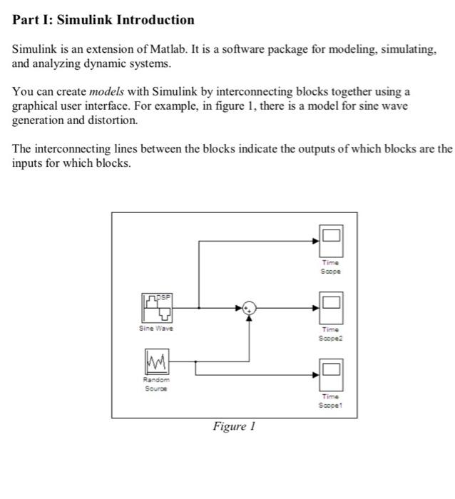
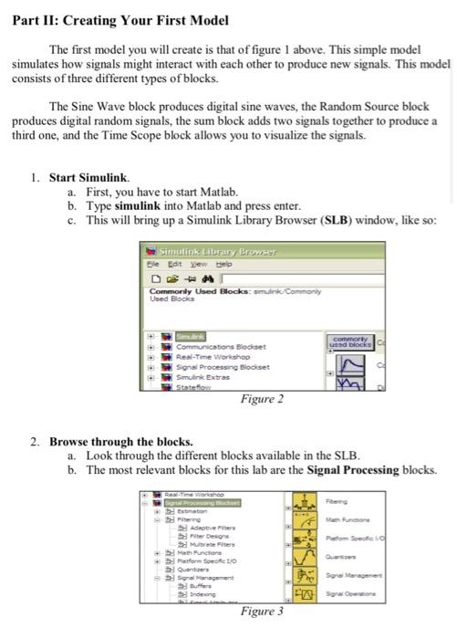
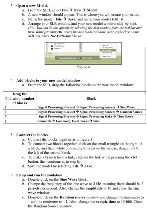
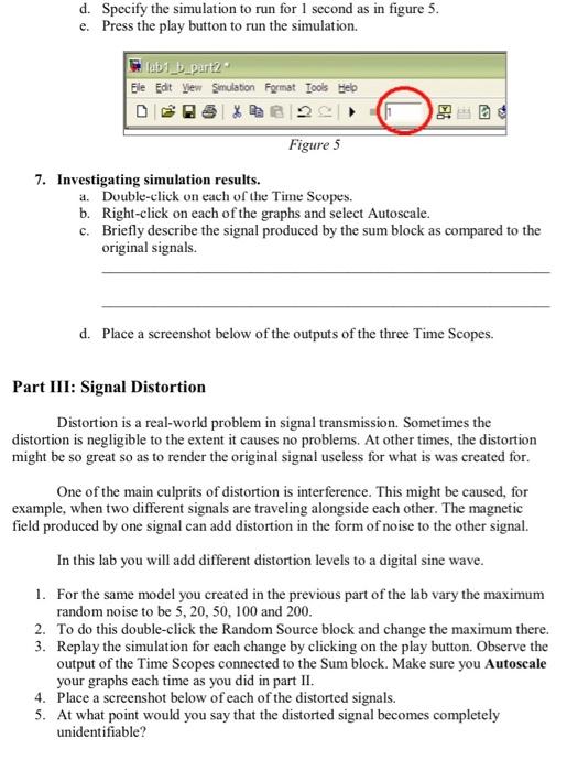
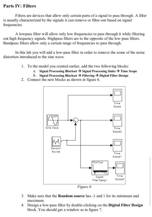
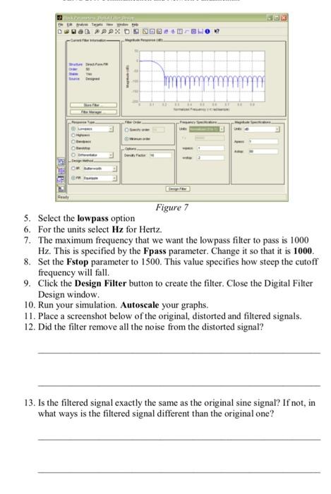
Part I: Simulink Introduction Simulink is an extension of Matlab. It is a software package for modeling, simulating, and analyzing dynamic systems. You can create models with Simulink by interconnecting blocks together using a graphical user interface. For example, in figure 1, there is a model for sine wave generation and distortion. The interconnecting lines between the blocks indicate the outputs of which blocks are the inputs for which blocks. Time Scope PSP Sine Wave Time Socce2 Random Soure Time Socet Figure 1 Part II: Creating Your First Model The first model you will create is that of figure 1 above. This simple model simulates how signals might interact with each other to produce new signals. This model consists of three different types of blocks. The Sine Wave block produces digital sine waves, the Random Source block produces digital random signals, the sum block adds two signals together to produce a third one, and the Time Scope block allows you to visualize the signals. 1. Start Simulink. a. First, you have to start Matlab. b. Type simulink into Matlab and press enter. c. This will bring up a Simulink Library Browser (SLB) window, like so: Simulinkbrary Browser Ele Edit wel DAN Commonly used Blocks muink Commonly Comory and blocks Communications Blocket Real-Time Workshop Signal Processing Blockset Simulink Extras Figure 2 2. Browse through the blocks. a. Look through the different blocks available in the SLB. b. The most relevant blocks for this lab are the Signal Processing blocks. erine Adaptives + Math Functions +5latform Socket Quentes >> Se Management uffer trene Figure 3 3. Open a new Model. a. From the SLB, select File New Model b. A new window should appear. This is where you will create your model. c. Name the model: File Save and name your model lab1_b d. Arrange your SLB window and your new model window side-by-side. Hint: You can do this quickly by selecting the SLB window from the taskbar and then, while pressing ctrl , select the new model window. Next, right click on the SLB and select Tile Vertically like so: Figure 4 4. Add blocks to your new model window. a. From the SLB, drag the following blocks to the new model window: Drag the following number of blocks 1 1 3 1 Block Signal Processing Blockset Signal Processing Sources Sine Wave Signal Processing Blockset Signal Processing Sources Random Source Signal Processing Blockset Signal Processing Sinks + Time Scope Simulink Commonly Used Blocks Sum 5. Connect the blocks. a. Connect the blocks together as in figure I. b. To connect two blocks together, click on the small triangle on the right of a block, and then, while continuing to press on the mouse, drag a link to the left of the second block. c. To make a branch from a link, click on the link while pressing the ctrl button, then continue as in step b. d. Save the model by selecting File Save. 6. Setup and run the simlation. a. Double-click on the Sine Wave block. b. Change the frequency of the sine wave to 2 Hz, meaning there should be 2 periods per second. Also change the amplitude to 10 and close the sine wave window. c. Double-click on the Random source window and change the maximum to I and the minimum to -1. Also, change the sample time to 1/1000. Close the Random Source window. d. Specify the simulation to run for 1 second as in figure 5. e. Press the play button to run the simulation. lab1_b.part2 Ele Edt View Simulation Format Tools Heb Elt Figure 5 7. Investigating simulation results. a. Double-click on each of the Time Scopes. b. Right click on each of the graphs and select Autoscale. c. Briefly describe the signal produced by the sum block as compared to the original signals. d. Place a screenshot below of the outputs of the three Time Scopes. Part III: Signal Distortion Distortion is a real-world problem in signal transmission. Sometimes the distortion is negligible to the extent it causes no problems. At other times, the distortion might be so great so as to render the original signal useless for what is was created for. One of the main culprits of distortion is interference. This might be caused, for example, when two different signals are traveling alongside each other. The magnetic field produced by one signal can add distortion in the form of noise to the other signal. In this lab you will add different distortion levels to a digital sine wave. 1. For the same model you created in the previous part of the lab vary the maximum random noise to be 5, 20, 50, 100 and 200. 2. To do this double-click the Random Source block and change the maximum there. 3. Replay the simulation for each change by clicking on the play button. Observe the output of the Time Scopes connected to the Sum block. Make sure you Autoscale your graphs each time as you did in part II. 4. Place a screenshot below of each of the distorted signals. 5. At what point would you say that the distorted signal becomes completely unidentifiable? Parts IV: Filters Filters are devices that allow only certain parts of a signal to pass through. A filter is usually characterized by the signals it can remove or filter-out based on signal frequencies. A lowpass filter will allow only low frequencies to pass through it while filtering out high frequency signals. Highpass filters are to the opposite of the low-pass filters. Bandpass filters allow only a certain range of frequencies to pass through. In this lab you will add a low-pass filter in order to remove the some of the noise distortion introduced to the sine wave. 1. To the model you created earlier, add the two following blocks: a. Signal Processing Blockset Signal Processing Sinks Time Scope b. Signal Processing Blockset Filtering Digital Filter Design 2. Connect the new blocks as shown in figure 6. Time Soepe psp Sine Wave Time Socce2 Random Souro Time Soopet FDATORI Time Scope Digital Filter Design Figure 6 3. Make sure that the Random source has -1 and 1 for its minimum and maximum 4. Design a low-pass filter by double-clicking on the Digital Filter Design block. You should get a window as in figure 7. - Figure 7 5. Select the lowpass option 6. For the units select Hz for Hertz. 7. The maximum frequency that we want the lowpass filter to pass is 1000 Hz. This is specified by the Fpass parameter. Change it so that it is 1000 8. Set the Fstop parameter to 1500. This value specifies how steep the cutoff frequency will fall 9. Click the Design Filter button to create the filter. Close the Digital Filter Design window. 10. Run your simulation. Autoscale your graphs. 11. Place a screenshot below of the original, distorted and filtered signals. 12. Did the filter remove all the noise from the distorted signal? 13. Is the filtered signal exactly the same as the original sine signal? If not, in what ways is the filtered signal different than the original one? Part I: Simulink Introduction Simulink is an extension of Matlab. It is a software package for modeling, simulating, and analyzing dynamic systems. You can create models with Simulink by interconnecting blocks together using a graphical user interface. For example, in figure 1, there is a model for sine wave generation and distortion. The interconnecting lines between the blocks indicate the outputs of which blocks are the inputs for which blocks. Time Scope PSP Sine Wave Time Socce2 Random Soure Time Socet Figure 1 Part II: Creating Your First Model The first model you will create is that of figure 1 above. This simple model simulates how signals might interact with each other to produce new signals. This model consists of three different types of blocks. The Sine Wave block produces digital sine waves, the Random Source block produces digital random signals, the sum block adds two signals together to produce a third one, and the Time Scope block allows you to visualize the signals. 1. Start Simulink. a. First, you have to start Matlab. b. Type simulink into Matlab and press enter. c. This will bring up a Simulink Library Browser (SLB) window, like so: Simulinkbrary Browser Ele Edit wel DAN Commonly used Blocks muink Commonly Comory and blocks Communications Blocket Real-Time Workshop Signal Processing Blockset Simulink Extras Figure 2 2. Browse through the blocks. a. Look through the different blocks available in the SLB. b. The most relevant blocks for this lab are the Signal Processing blocks. erine Adaptives + Math Functions +5latform Socket Quentes >> Se Management uffer trene Figure 3 3. Open a new Model. a. From the SLB, select File New Model b. A new window should appear. This is where you will create your model. c. Name the model: File Save and name your model lab1_b d. Arrange your SLB window and your new model window side-by-side. Hint: You can do this quickly by selecting the SLB window from the taskbar and then, while pressing ctrl , select the new model window. Next, right click on the SLB and select Tile Vertically like so: Figure 4 4. Add blocks to your new model window. a. From the SLB, drag the following blocks to the new model window: Drag the following number of blocks 1 1 3 1 Block Signal Processing Blockset Signal Processing Sources Sine Wave Signal Processing Blockset Signal Processing Sources Random Source Signal Processing Blockset Signal Processing Sinks + Time Scope Simulink Commonly Used Blocks Sum 5. Connect the blocks. a. Connect the blocks together as in figure I. b. To connect two blocks together, click on the small triangle on the right of a block, and then, while continuing to press on the mouse, drag a link to the left of the second block. c. To make a branch from a link, click on the link while pressing the ctrl button, then continue as in step b. d. Save the model by selecting File Save. 6. Setup and run the simlation. a. Double-click on the Sine Wave block. b. Change the frequency of the sine wave to 2 Hz, meaning there should be 2 periods per second. Also change the amplitude to 10 and close the sine wave window. c. Double-click on the Random source window and change the maximum to I and the minimum to -1. Also, change the sample time to 1/1000. Close the Random Source window. d. Specify the simulation to run for 1 second as in figure 5. e. Press the play button to run the simulation. lab1_b.part2 Ele Edt View Simulation Format Tools Heb Elt Figure 5 7. Investigating simulation results. a. Double-click on each of the Time Scopes. b. Right click on each of the graphs and select Autoscale. c. Briefly describe the signal produced by the sum block as compared to the original signals. d. Place a screenshot below of the outputs of the three Time Scopes. Part III: Signal Distortion Distortion is a real-world problem in signal transmission. Sometimes the distortion is negligible to the extent it causes no problems. At other times, the distortion might be so great so as to render the original signal useless for what is was created for. One of the main culprits of distortion is interference. This might be caused, for example, when two different signals are traveling alongside each other. The magnetic field produced by one signal can add distortion in the form of noise to the other signal. In this lab you will add different distortion levels to a digital sine wave. 1. For the same model you created in the previous part of the lab vary the maximum random noise to be 5, 20, 50, 100 and 200. 2. To do this double-click the Random Source block and change the maximum there. 3. Replay the simulation for each change by clicking on the play button. Observe the output of the Time Scopes connected to the Sum block. Make sure you Autoscale your graphs each time as you did in part II. 4. Place a screenshot below of each of the distorted signals. 5. At what point would you say that the distorted signal becomes completely unidentifiable? Parts IV: Filters Filters are devices that allow only certain parts of a signal to pass through. A filter is usually characterized by the signals it can remove or filter-out based on signal frequencies. A lowpass filter will allow only low frequencies to pass through it while filtering out high frequency signals. Highpass filters are to the opposite of the low-pass filters. Bandpass filters allow only a certain range of frequencies to pass through. In this lab you will add a low-pass filter in order to remove the some of the noise distortion introduced to the sine wave. 1. To the model you created earlier, add the two following blocks: a. Signal Processing Blockset Signal Processing Sinks Time Scope b. Signal Processing Blockset Filtering Digital Filter Design 2. Connect the new blocks as shown in figure 6. Time Soepe psp Sine Wave Time Socce2 Random Souro Time Soopet FDATORI Time Scope Digital Filter Design Figure 6 3. Make sure that the Random source has -1 and 1 for its minimum and maximum 4. Design a low-pass filter by double-clicking on the Digital Filter Design block. You should get a window as in figure 7. - Figure 7 5. Select the lowpass option 6. For the units select Hz for Hertz. 7. The maximum frequency that we want the lowpass filter to pass is 1000 Hz. This is specified by the Fpass parameter. Change it so that it is 1000 8. Set the Fstop parameter to 1500. This value specifies how steep the cutoff frequency will fall 9. Click the Design Filter button to create the filter. Close the Digital Filter Design window. 10. Run your simulation. Autoscale your graphs. 11. Place a screenshot below of the original, distorted and filtered signals. 12. Did the filter remove all the noise from the distorted signal? 13. Is the filtered signal exactly the same as the original sine signal? If not, in what ways is the filtered signal different than the original one