Use python to work through the example given in 6.2.1 Using Matlab to Fit Data for the English Boarding School example.
6.2.1 Using Matlab to Fit Data for the English Boarding School


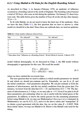
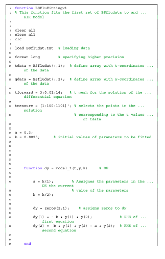
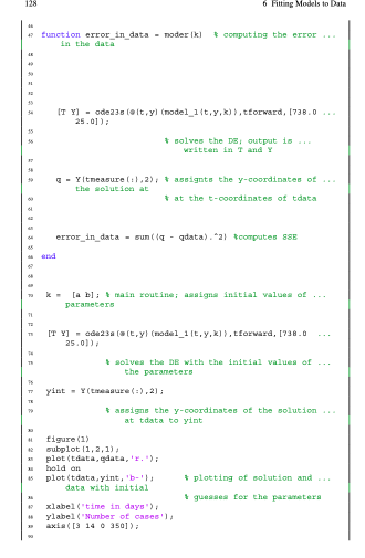
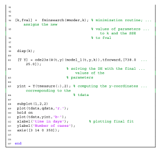
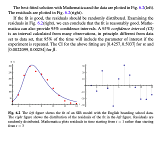
6.2.1 Using Matlab to Fit Data for the English Boarding School As described in Chap. 2. in January February 1978, an epidemic of influenza occurred in a boarding school in the north of England. The boarding school housed a total of 763 bays, who were at risk during the epidemic. On January 22, three boys were sick. The table below gives the number of boys ill on the oth day after January 22 ( 11) To fit with Matlab, we do not need to know the final size of the epidemic. Once we have the data (Table 6.1), the first question that we have to answer is, what model we should fit to the data? Since these are outbreak data, we need an epidemic Table 6.1 Daily number influmea infected boys Day No infected Day No, infected 3 25 9 192 75 10 5 227 11 71 296 12 25 7 255 13 & 236 14 Data taken from "Influenza in a Boarding School," British Medical Journal, 4 March 1978 model without demography. As we discussed in Chap. 2. the SIR model without demography is appropriate for this case. We recall the model: $(8) - BS(1)(:), (6.1) ric) =B5(1)() - al(e), where we have omitted the recovered class. The next question that we need to address is which model parameters we should fit and which we should pre-estimate and fix. Potentially, we can fit a. B, and the initial conditions four parameters altogether. We can pre-estimate from the duration of infectiousness, and the two initial conditions from the given data. For instance, we know from the data that (3) = 25, and therefore (3) = 738. The dur- ation of infectiousness is 2-4 days, so we may take a=0.3. Even if we plan to fit all these parameters, pre-estimating what we can is useful with the initial guess of the parameters. In addition, to derive the initial guesses for the remaining parameters before using Matlab to fit, we may use Mathematica's Manipulate command. In Mathematica, we can fix (3), 7(3), and to the above values and manipulate" to obtain a good agreement with the data. Say we set the value p = 0.0025. With these initial values, we may use Matlab to fit. Below is the Matlab code used for the fitting. Eunetion BSPluiting! 2. This function tits the first set of escludata to and SIR model clear all elose all ele load Estludat.txt loading data 1 Cornat long specifying higher precision tdata - Berludat (:,1); define array with t-coordinates ... DE the data is data - Bsf ludat (:,2), define array with y-coordinates ... of the data 19tforward - 3:0.01:14 t mesh for the solution of the difcerential equation treasure - (1:100:11011'; selects the points in the ... solution corresponding to the values... o data 2.0.0025; initial values of parameters to be fitted 15 Lunetion dy model_116,y,k) Assignes the parameters in the ... DE the current value of the parameters bk (2) dy - zeros(2,1) * assigns zeros to dy dy 111 --by) y121 RHS of first equation dy 12) - Dy(1) y(2) ay(2); RHS of second equation IF 128 6 Fitting Models to Data 42 function error_in_data - noder kl in the data computing the error 19 45 IT Y) - ode235 leit yl (model_1{t,y,k) ),tforward, 1738.0... 25.01) solves the De output is written in T and y - Yitmeasure 1:1, 2); assignts the y-coordinates of ... the solution at at the t-coordinates of tdata error_in_data - sun(( - adata). 21 tcomputes SSE 65 end k. [a b] ; main routine; assigna initial values of ... parameters 71 IT Y] - cda23a ((tyl (nade1_116,y,X1),tforward. [736.0 25.01) solves the DE with the initial values of ... the parameters yint - Y/tmeasure (-),21; assigns the y-coordinates of the solution... at tdata to yint figure (2) subplot 11,2,1); plot(tdata, data,'.); hold on plot (tdata, yint, 'b- * plotting of solution and ... data with initial guesse cor the parameters xlabel('tine in days) ylabel("Number of case'l axia (3 14 O 350]); 45 42 9 [k, Eval] . insearch (oder,k); minimisation routine; 25signs the new * values of parameters ... to k and the sea ta Eval disp(); IT Y) - de 23 fett,yl (nodel_11t.y, kl),tforward, 1738.0 25.0]); * solving the be with the final values of the parameters yint - Y(tmeasure(+),21: * computing the y-coordinates corresponding to the data subplot 11,2,2) plot (tdata, adata, 'r. '); hold on plot(tdata yint, 'b' xlabel('time in days"); plotting final fit ylabeluber of cases'; axia [3 14 O 350]); 116 111 112 111 115 Hend The best-fitted solution with Mathematica and the data are plotted in Fig.6.2(left). The residuals are plotted in Fig. 6.2(right), If the fit is good, the residuals should be randomly distributed. Examining the residuals in Fig. 6.2 (right), we can conclude that the fit is reasonably good. Mathe- matica can also provide 95% confidence intervals. A 95% confidence interval (CI) is an interval calculated from many observations, in principle different from data set to data set, that 95% of the time will include the parameter of interest if the experiment is repeated. The Cl for the above fitting are (0.4257,0.5037for and (0.0022099, 0.00254 for B. Fig. 6.2 The le figure shows the fit of an SIR model with the English boarding school data The right figure shows the distribution of the residuals of the fit in the left figure Residuals are randomly distributed. Mathematica plots residuals in time starting from i = 1 rather than starting from - 3 6.2.1 Using Matlab to Fit Data for the English Boarding School As described in Chap. 2. in January February 1978, an epidemic of influenza occurred in a boarding school in the north of England. The boarding school housed a total of 763 bays, who were at risk during the epidemic. On January 22, three boys were sick. The table below gives the number of boys ill on the oth day after January 22 ( 11) To fit with Matlab, we do not need to know the final size of the epidemic. Once we have the data (Table 6.1), the first question that we have to answer is, what model we should fit to the data? Since these are outbreak data, we need an epidemic Table 6.1 Daily number influmea infected boys Day No infected Day No, infected 3 25 9 192 75 10 5 227 11 71 296 12 25 7 255 13 & 236 14 Data taken from "Influenza in a Boarding School," British Medical Journal, 4 March 1978 model without demography. As we discussed in Chap. 2. the SIR model without demography is appropriate for this case. We recall the model: $(8) - BS(1)(:), (6.1) ric) =B5(1)() - al(e), where we have omitted the recovered class. The next question that we need to address is which model parameters we should fit and which we should pre-estimate and fix. Potentially, we can fit a. B, and the initial conditions four parameters altogether. We can pre-estimate from the duration of infectiousness, and the two initial conditions from the given data. For instance, we know from the data that (3) = 25, and therefore (3) = 738. The dur- ation of infectiousness is 2-4 days, so we may take a=0.3. Even if we plan to fit all these parameters, pre-estimating what we can is useful with the initial guess of the parameters. In addition, to derive the initial guesses for the remaining parameters before using Matlab to fit, we may use Mathematica's Manipulate command. In Mathematica, we can fix (3), 7(3), and to the above values and manipulate" to obtain a good agreement with the data. Say we set the value p = 0.0025. With these initial values, we may use Matlab to fit. Below is the Matlab code used for the fitting. Eunetion BSPluiting! 2. This function tits the first set of escludata to and SIR model clear all elose all ele load Estludat.txt loading data 1 Cornat long specifying higher precision tdata - Berludat (:,1); define array with t-coordinates ... DE the data is data - Bsf ludat (:,2), define array with y-coordinates ... of the data 19tforward - 3:0.01:14 t mesh for the solution of the difcerential equation treasure - (1:100:11011'; selects the points in the ... solution corresponding to the values... o data 2.0.0025; initial values of parameters to be fitted 15 Lunetion dy model_116,y,k) Assignes the parameters in the ... DE the current value of the parameters bk (2) dy - zeros(2,1) * assigns zeros to dy dy 111 --by) y121 RHS of first equation dy 12) - Dy(1) y(2) ay(2); RHS of second equation IF 128 6 Fitting Models to Data 42 function error_in_data - noder kl in the data computing the error 19 45 IT Y) - ode235 leit yl (model_1{t,y,k) ),tforward, 1738.0... 25.01) solves the De output is written in T and y - Yitmeasure 1:1, 2); assignts the y-coordinates of ... the solution at at the t-coordinates of tdata error_in_data - sun(( - adata). 21 tcomputes SSE 65 end k. [a b] ; main routine; assigna initial values of ... parameters 71 IT Y] - cda23a ((tyl (nade1_116,y,X1),tforward. [736.0 25.01) solves the DE with the initial values of ... the parameters yint - Y/tmeasure (-),21; assigns the y-coordinates of the solution... at tdata to yint figure (2) subplot 11,2,1); plot(tdata, data,'.); hold on plot (tdata, yint, 'b- * plotting of solution and ... data with initial guesse cor the parameters xlabel('tine in days) ylabel("Number of case'l axia (3 14 O 350]); 45 42 9 [k, Eval] . insearch (oder,k); minimisation routine; 25signs the new * values of parameters ... to k and the sea ta Eval disp(); IT Y) - de 23 fett,yl (nodel_11t.y, kl),tforward, 1738.0 25.0]); * solving the be with the final values of the parameters yint - Y(tmeasure(+),21: * computing the y-coordinates corresponding to the data subplot 11,2,2) plot (tdata, adata, 'r. '); hold on plot(tdata yint, 'b' xlabel('time in days"); plotting final fit ylabeluber of cases'; axia [3 14 O 350]); 116 111 112 111 115 Hend The best-fitted solution with Mathematica and the data are plotted in Fig.6.2(left). The residuals are plotted in Fig. 6.2(right), If the fit is good, the residuals should be randomly distributed. Examining the residuals in Fig. 6.2 (right), we can conclude that the fit is reasonably good. Mathe- matica can also provide 95% confidence intervals. A 95% confidence interval (CI) is an interval calculated from many observations, in principle different from data set to data set, that 95% of the time will include the parameter of interest if the experiment is repeated. The Cl for the above fitting are (0.4257,0.5037for and (0.0022099, 0.00254 for B. Fig. 6.2 The le figure shows the fit of an SIR model with the English boarding school data The right figure shows the distribution of the residuals of the fit in the left figure Residuals are randomly distributed. Mathematica plots residuals in time starting from i = 1 rather than starting from - 3
