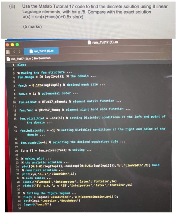
Use the Matlab Tutorial 17 code to find the discrete solution using 8 linear Lagrange elements, with h= /8. Compare with the exact solution u(x) = sin(x)+cos(x)+0.5x sin(x). (5 marks) 5 7 9 11 run_Tut 17 (1).m run Tues (1). run_Tut17 (1).m) No Selection 1 clear 2 3 X Making the fem structure ... 4 fem.Omega - [6 log(2opi)); * the domain ... fem.h - 0.1256log(24pl); * desired mesh size ... 8 fom.p = 1; X polynomial order ... 10 fen.elemat - Tut17_clonat; X element matrix function ... 12 fem.func - Tut17_func; * element right hand side function ... 13 14 fem.adirichlet-cos(1); * setting Dirichlet conditions at the left end point of the domain ... 16 fem.bdirichlet = -1; * setting Dirichlet conditions at the right end point of the domain ... 17 18 fem.quadrulouh; selecting the desired quadrature rule ... 20 (u * T] = fon_solver (fem); * solving ... 21 22 X making plot ... 23 X the analytic solution ... 24 plot([0:0.01.log(201)].-cos(exp((0:0.01:log(20p)])), 'b', 'Linewidth', 2); hold 25 X numerical solution 26 plot(x,u,'o-.k', 'LineWidth',1); 27 % axes labels ... 28 xlabel('slOmegas', 'interpreter","latox','fonteize', 16) 29 ylabel('s' u_h, N; u MS', 'interpreter', 'latex','fontsize', 14) 30 31 x Setting the figure legend ... 32 hlegi legend( "solution)', 'u_h(approximation, p-1)'); 30 set(hlegi, 'Location', 'Southwest) 34 legend('boxoff') 35 15 19 Use the Matlab Tutorial 17 code to find the discrete solution using 8 linear Lagrange elements, with h= /8. Compare with the exact solution u(x) = sin(x)+cos(x)+0.5x sin(x). (5 marks) 5 7 9 11 run_Tut 17 (1).m run Tues (1). run_Tut17 (1).m) No Selection 1 clear 2 3 X Making the fem structure ... 4 fem.Omega - [6 log(2opi)); * the domain ... fem.h - 0.1256log(24pl); * desired mesh size ... 8 fom.p = 1; X polynomial order ... 10 fen.elemat - Tut17_clonat; X element matrix function ... 12 fem.func - Tut17_func; * element right hand side function ... 13 14 fem.adirichlet-cos(1); * setting Dirichlet conditions at the left end point of the domain ... 16 fem.bdirichlet = -1; * setting Dirichlet conditions at the right end point of the domain ... 17 18 fem.quadrulouh; selecting the desired quadrature rule ... 20 (u * T] = fon_solver (fem); * solving ... 21 22 X making plot ... 23 X the analytic solution ... 24 plot([0:0.01.log(201)].-cos(exp((0:0.01:log(20p)])), 'b', 'Linewidth', 2); hold 25 X numerical solution 26 plot(x,u,'o-.k', 'LineWidth',1); 27 % axes labels ... 28 xlabel('slOmegas', 'interpreter","latox','fonteize', 16) 29 ylabel('s' u_h, N; u MS', 'interpreter', 'latex','fontsize', 14) 30 31 x Setting the figure legend ... 32 hlegi legend( "solution)', 'u_h(approximation, p-1)'); 30 set(hlegi, 'Location', 'Southwest) 34 legend('boxoff') 35 15 19