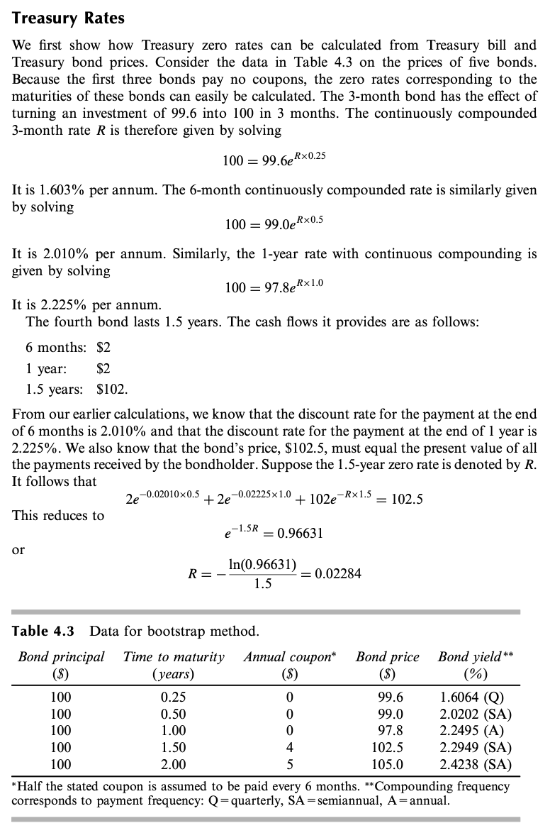
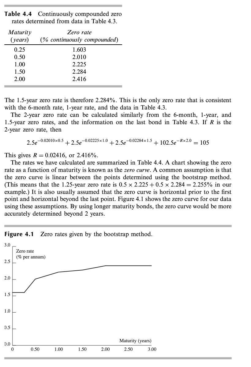
Using Excel, replicate the example using data in Table 4.3 to produce the output shown in Table 4.4 and Figure 4.1.

Treasury Rates We first show how Treasury zero rates can be calculated from Treasury bill and Treasury bond prices. Consider the data in Table 4.3 on the prices of five bonds. Because the first three bonds pay no coupons, the zero rates corresponding to the maturities of these bonds can easily be calculated. The 3-month bond has the effect of turning an investment of 99.6 into 100 in 3 months. The continuously compounded 3-month rate R is therefore given by solving 100 = 99.6eRx0.25 It is 1.603% per annum. The 6-month continuously compounded rate is similarly given by solving 100 = 99.0eRx0.5 1 year: It is 2.010% per annum. Similarly, the 1-year rate with continuous compounding is given by solving 100 = 97.8eRx1.0 It is 2.225% per annum. The fourth bond lasts 1.5 years. The cash flows it provides are as follows: 6 months: $2 $2 1.5 years: $102. From our earlier calculations, we know that the discount rate for the payment at the end of 6 months is 2.010% and that the discount rate for the payment at the end of 1 year is 2.225%. We also know that the bond's price, $102.5, must equal the present value of all the payments received by the bondholder. Suppose the 1.5-year zero rate is denoted by R. It follows that + 2e -0.02225x1.0 + 102e = 102.5 This reduces to = 0.96631 or In(0.96631) R= = 0.02284 1.5 2e-0.02010x0.5 e-Rx1.5 e-1.5R Table 4.3 Data for bootstrap method. Bond principal Time to maturity Annual coupon* Bond price Bond yield** ($) (years) ($) ($) (%) 100 0.25 0 99.6 1.6064 (Q) 100 0.50 0 99.0 2.0202 (SA) 100 1.00 0 97.8 2.2495 (A) 100 1.50 4 102.5 2.2949 (SA) 100 2.00 5 105.0 2.4238 (SA) * Half the stated coupon is assumed to be paid every 6 months. **Compounding frequency corresponds to payment frequency: Q=quarterly, SA =semiannual, A=annual. Table 4.4 Continuously compounded zero rates determined from data in Table 4.3. Maturity Zero rate (years) (% continuously compounded) 0.25 1.603 0.50 2.010 1.00 2.225 1.50 2.284 2.00 2.416 The 1.5-year zero rate is therefore 2.284%. This is the only zero rate that is consistent with the 6-month rate, 1-year rate, and the data in Table 4.3. The 2-year zero rate can be calculated similarly from the 6-month, 1-year, and 1.5-year zero rates, and the information on the last bond in Table 4.3. If R is the 2-year zero rate, then 2.5e -0.02010x0.5 +2.5e -0.02225x1.0 +2.5e -0.02284x1.5 + 102.5e -Rx2.0 = 105 This gives R = 0.02416, or 2.416%. The rates we have calculated are summarized in Table 4.4. A chart showing the zero rate as a function of maturity is known as the zero curve. A common assumption is that the zero curve is linear between the points determined using the bootstrap method. (This means that the 1.25-year zero rate is 0.5 x 2.225 +0.5 x 2.284 = 2.255% in our example.) It is also usually assumed that the zero curve is horizontal prior to the first point and horizontal beyond the last point. Figure 4.1 shows the zero curve for our data using these assumptions. By using longer maturity bonds, the zero curve would be more accurately determined beyond 2 years. Figure 4.1 Zero rates given by the bootstrap method. 3.0 Zero rate (% per annum) 2.5 2.0 1.5 1.0 0.5 0.0 0 Maturity (years) 2.50 3.00 0.50 1.00 1.50 2.00 Treasury Rates We first show how Treasury zero rates can be calculated from Treasury bill and Treasury bond prices. Consider the data in Table 4.3 on the prices of five bonds. Because the first three bonds pay no coupons, the zero rates corresponding to the maturities of these bonds can easily be calculated. The 3-month bond has the effect of turning an investment of 99.6 into 100 in 3 months. The continuously compounded 3-month rate R is therefore given by solving 100 = 99.6eRx0.25 It is 1.603% per annum. The 6-month continuously compounded rate is similarly given by solving 100 = 99.0eRx0.5 1 year: It is 2.010% per annum. Similarly, the 1-year rate with continuous compounding is given by solving 100 = 97.8eRx1.0 It is 2.225% per annum. The fourth bond lasts 1.5 years. The cash flows it provides are as follows: 6 months: $2 $2 1.5 years: $102. From our earlier calculations, we know that the discount rate for the payment at the end of 6 months is 2.010% and that the discount rate for the payment at the end of 1 year is 2.225%. We also know that the bond's price, $102.5, must equal the present value of all the payments received by the bondholder. Suppose the 1.5-year zero rate is denoted by R. It follows that + 2e -0.02225x1.0 + 102e = 102.5 This reduces to = 0.96631 or In(0.96631) R= = 0.02284 1.5 2e-0.02010x0.5 e-Rx1.5 e-1.5R Table 4.3 Data for bootstrap method. Bond principal Time to maturity Annual coupon* Bond price Bond yield** ($) (years) ($) ($) (%) 100 0.25 0 99.6 1.6064 (Q) 100 0.50 0 99.0 2.0202 (SA) 100 1.00 0 97.8 2.2495 (A) 100 1.50 4 102.5 2.2949 (SA) 100 2.00 5 105.0 2.4238 (SA) * Half the stated coupon is assumed to be paid every 6 months. **Compounding frequency corresponds to payment frequency: Q=quarterly, SA =semiannual, A=annual. Table 4.4 Continuously compounded zero rates determined from data in Table 4.3. Maturity Zero rate (years) (% continuously compounded) 0.25 1.603 0.50 2.010 1.00 2.225 1.50 2.284 2.00 2.416 The 1.5-year zero rate is therefore 2.284%. This is the only zero rate that is consistent with the 6-month rate, 1-year rate, and the data in Table 4.3. The 2-year zero rate can be calculated similarly from the 6-month, 1-year, and 1.5-year zero rates, and the information on the last bond in Table 4.3. If R is the 2-year zero rate, then 2.5e -0.02010x0.5 +2.5e -0.02225x1.0 +2.5e -0.02284x1.5 + 102.5e -Rx2.0 = 105 This gives R = 0.02416, or 2.416%. The rates we have calculated are summarized in Table 4.4. A chart showing the zero rate as a function of maturity is known as the zero curve. A common assumption is that the zero curve is linear between the points determined using the bootstrap method. (This means that the 1.25-year zero rate is 0.5 x 2.225 +0.5 x 2.284 = 2.255% in our example.) It is also usually assumed that the zero curve is horizontal prior to the first point and horizontal beyond the last point. Figure 4.1 shows the zero curve for our data using these assumptions. By using longer maturity bonds, the zero curve would be more accurately determined beyond 2 years. Figure 4.1 Zero rates given by the bootstrap method. 3.0 Zero rate (% per annum) 2.5 2.0 1.5 1.0 0.5 0.0 0 Maturity (years) 2.50 3.00 0.50 1.00 1.50 2.00