

Question
Using Python: curve80.txt contains: 3.4447005e+00 -8.8011696e-01 4.7580645e+00 4.6491228e-01 6.4170507e+00 3.7397661e+00 5.7949309e+00 3.0087719e+00 7.7304147e+00 2.9210526e+00 7.8225806e+00 4.1491228e+00 7.7304147e+00 3.3888889e+00 7.7764977e+00 3.7105263e+00 8.6751152e+00 2.9795322e+00 6.4631336e+00 3.9736842e+00 5.1267281e+00
Using Python:
curve80.txt contains:
3.4447005e+00 -8.8011696e-01 4.7580645e+00 4.6491228e-01 6.4170507e+00 3.7397661e+00 5.7949309e+00 3.0087719e+00 7.7304147e+00 2.9210526e+00 7.8225806e+00 4.1491228e+00 7.7304147e+00 3.3888889e+00 7.7764977e+00 3.7105263e+00 8.6751152e+00 2.9795322e+00 6.4631336e+00 3.9736842e+00 5.1267281e+00 1.1403509e-01 6.7396313e+00 4.1491228e+00 3.1451613e+00 -5.0000000e-01 9.1589862e+00 4.0906433e+00 8.2373272e+00 2.8040936e+00 4.8041475e+00 -5.0000000e-01 3.5714286e-01 -1.4941520e+00 8.0069124e+00 4.0321637e+00 2.2465438e+00 -7.6315789e-01 6.7626728e+00 4.4122807e+00 5.0115207e+00 1.0204678e+00 8.7211982e+00 3.0087719e+00 1.6935484e+00 -6.7543860e-01 4.8502304e+00 3.7719298e-01 8.6059908e+00 4.6461988e+00 8.2142857e+00 4.1491228e+00 8.1797235e-01 -1.4649123e+00 5.7488479e+00 2.1023392e+00 6.7165899e+00 4.0321637e+00 2.0391705e+00 -9.9707602e-01 5.1036866e+00 1.8976608e+00 4.3433180e+00 5.8187135e-01 4.4815668e+00 -7.6315789e-01 7.3156682e+00 4.9385965e+00 8.5138249e+00 3.4473684e+00 9.0207373e+00 2.8625731e+00 5.4953917e+00 2.1023392e+00 6.0483871e+00 3.5935673e+00 4.5506912e+00 -7.6315789e-01 2.6843318e+00 -6.4619883e-01 6.8087558e+00 4.7046784e+00 1.7857143e+00 -1.3187135e+00 5.4723502e+00 1.7222222e+00 3.3755760e+00 -9.9707602e-01 7.7304147e+00 4.5584795e+00 6.7396313e+00 5.1432749e+00 4.2741935e+00 -1.0263158e+00 4.7811060e+00 1.5467836e+00 5.8870968e+00 2.4532164e+00 8.8133641e+00 4.1783626e+00 5.9101382e+00 3.6228070e+00 4.8502304e+00 7.8654971e-01 6.6013825e+00 4.4707602e+00 1.2557604e+00 -1.2309942e+00 4.1129032e+00 -9.6783626e-01 7.1774194e+00 2.8333333e+00 4.8271889e+00 -2.9532164e-01 2.9147465e+00 -1.0847953e+00 5.1728111e+00 1.6345029e+00 5.8410138e+00 2.8625731e+00 8.4907834e+00 2.3070175e+00 7.4078341e+00 3.7982456e+00 8.1797235e-01 -9.9707602e-01 7.2580645e-01 -4.7076023e-01 7.5921659e+00 4.1491228e+00 8.8133641e+00 3.4766082e+00 2.4769585e+00 -9.3859649e-01 4.5737327e+00 -1.1988304e-01 8.6751152e+00 3.7982456e+00 6.1635945e+00 2.6871345e+00 8.3525346e+00 3.5643275e+00 6.5783410e+00 4.5292398e+00 4.8271889e+00 6.6959064e-01 2.5230415e+00 -1.2309942e+00 2.4193548e-01 3.4795322e-01 6.2327189e+00 4.1783626e+00 8.7903226e+00 3.0380117e+00 2.2695853e+00 -1.0847953e+00 6.3709677e+00 6.1959064e+00 6.0253456e+00 3.0964912e+00
Given:
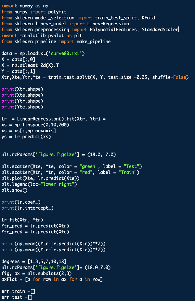
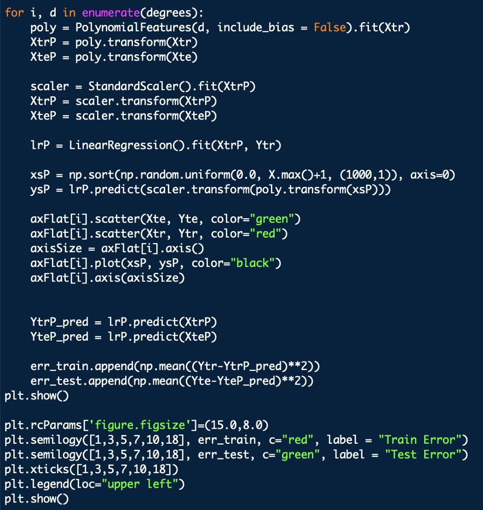
Outputs should look the like above graphs
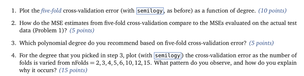
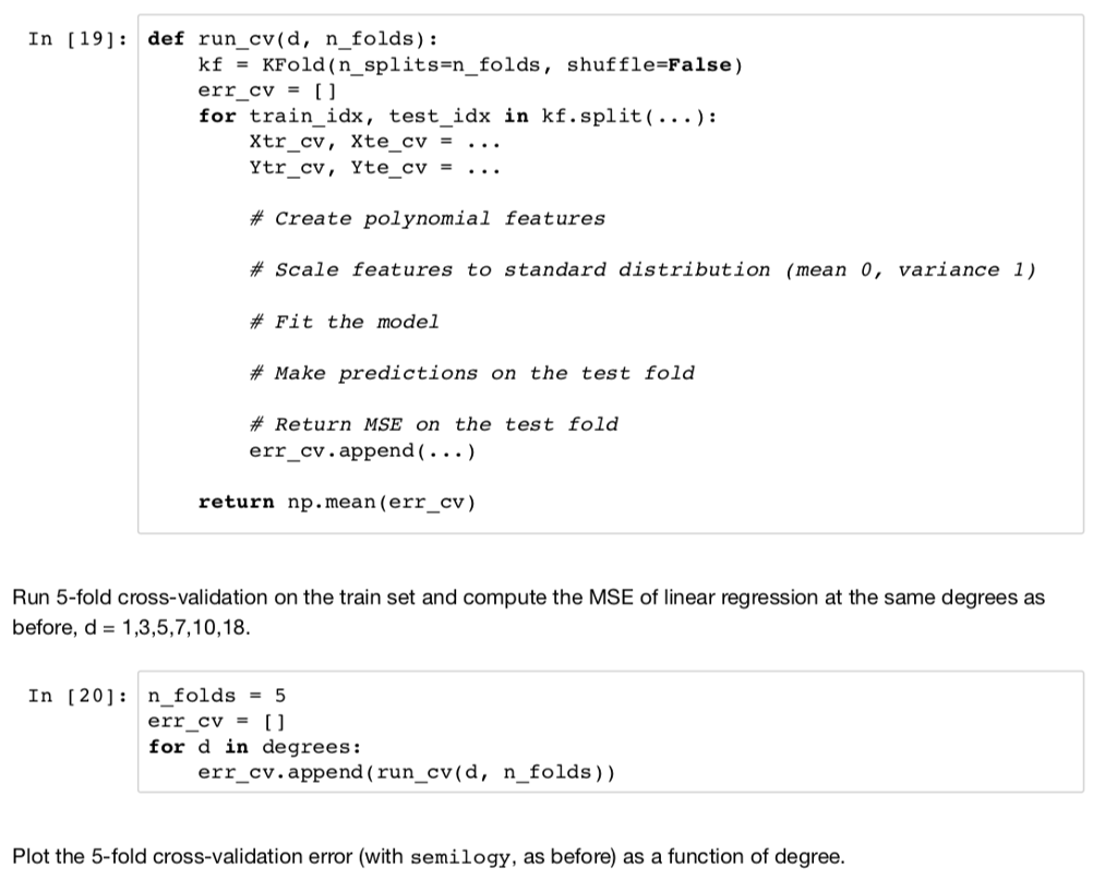
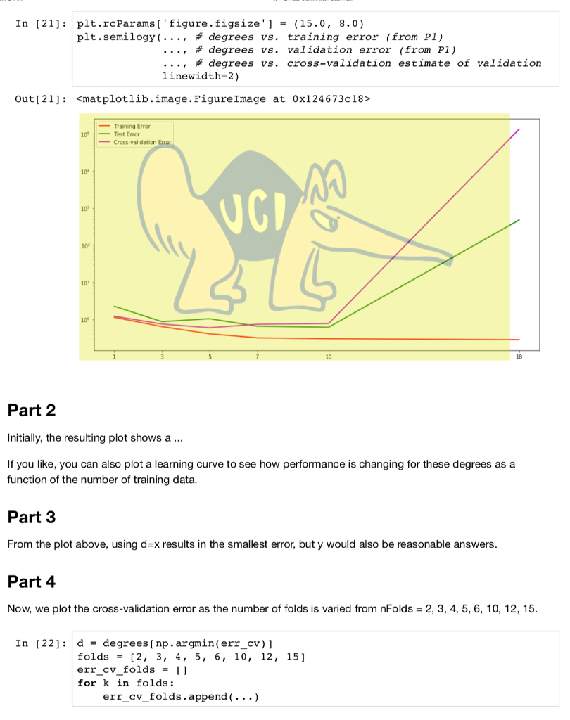
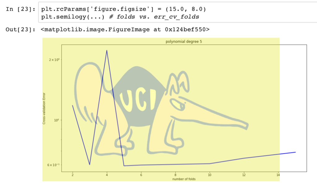
import numpy as np from numpy import polyfift from sklearn.model_selection import train test split, KFold from sklearn.linear_model import LinearRegression from sklearn.preprocessing import PolynomialFeatures, StandardScaler import matplotlib.pyplot as plt from sklearn.pipeline import make_pipeline data np.loadtxt('curve80.txt x - dataC:,0] X-np.atleast_2d(X).T Y data[:,1] Xtr,Xte,Ytr,Yte -train test split(X, Y, test _size -0.25, shuffle-False) print(Xtr.shape) print(Xte.shape) print(Ytr.shape) print(Yte.shape) Lr LinearRegressionO.fit(Xtr, Ytr) - xs np. linspace(0,10,200) xs = xs[.,np.newaxis] yslr.predict(xs) plt.rcParams ['figure.figsize']-(18.0, 7.0) pit , scatter(Xte, Yte, color= "green", label- "Test") plt.scatter(Xtr, Ytr, color"red", label-"Train") plt.plot(Xte, lr.predict(Xte)) plt.legend(loc-"lower right") plt.showO print(lr.coef_) print(lr.intercept_) Ir.fit(Xtr, Ytr) Ytr_predlr.predict(Xtr) Yte_predlr.predict(Xte) print(np.mean((Ytr-lr.predict(Xtr))**2)) print(np.mean ((Yte-1r.predict(Xte))**2)) degrees[1,3,5,7,10,18] plt.rcParamsD' figure.figsize']- (18.0,7.0) fig, ax -plt.subplots(2,3) axFlat [a for row in ax for a in row] err_train err_test for i, d in enumerate(degrees): poly - PolynomialFeatures(d, include_bias False).fit(Xtr) XtrP - poly.transform(Xtr) XteP = poly. transform(Xte) scaler = StandardScalero.fit(XtrP) XtrP -scaler.transform(XtrP) XteP-scaler. transform(XteP) LrP -LinearRegressionO.fit(XtrP, Ytr) xsP - np.sort(np.random.uniform(0.0, X.max)+1, (1000,1)), axis-0) ysP1rP.predict(scaler.transform(poly.transform(xsP))) axFlat[i].scatter(Xte, Yte, color-"green") axFlat[i].scatter(Xtr, Ytr, color-"red") axisSize -axFlat[i].axisO axFlat[i].plot(xsP, ysP, color='' black") axFlat[i].axis(axisSize) YtrP_pred- 1rP.predict(XtrP) Yter_pred lrP. predict(XteP) err_train.append(np.mean((Ytr-YtrP_pred)**2)) err_test.append(np.mean ((Yte-YteP_pred)**2)) plt.showO plt.rcParams'figure.figsize']-(15.0,8.0) plt.semilogyC [1 , 3, 5, 7, 10,18] , err-train, c"red", label- "Train Error") plt.semilogy([1,3,5,7,10,18], err_test, c-"green", label "Test Error") plt.xticks([1,3,5,7,10,18]) plt.legend(loc-"upper left") plt.show) 1. Plot the five-fold cross-validation error (with semilogy, as before) as a function of degree. (10 points) 2. How do the MSE estimates from five-fold cross-validation compare to the MSEs evaluated on the actual test data (Problem 1)? (5 points) 3. Which polynomial degree do you recommend based on five-fold cross-validation error? (5 points) 4. For the degree that you picked in step 3, plot (with semilogy the cross-validation error as the number of folds is varied from nFolds-2,3,4,5,6, 10,12,15. What pattern do you observe, and how do you explain why it occurs? (15 points) In [19]: def run cv(d, n_folds): kf- KFold (n-splits-n-folds, shuffle-False) err_cv- for train idx, test_idx in kf.split(...: Xtr cv, Xte cv - # Create polynomial features # Scale features to standard distribution (mean 0, variance 1) # Fit the model # Make predictions on the test fold # Return MSE on the test fold err_cv.append (. ..) return np.mean(err_ev) Run 5-fold cross-validation on the train set and compute the MSE of linear regression at the same degrees as before, d 1,3,5,7,10,18. In 201n folds 5 in degrees: err_cv.append (run_cv(d, n folds)) for d Plot the 5-fold cross-validation error (with semilogy, as before) as a function of degree. In [21]: plt.rcParams 'figure.figsize'] - (15.0, 8.0) pt.semi logy( ' #degrees vs. training error (from P1) , # degrees vs. validation error (from P1) , # degrees vs. cross-validation estimate of validation linewidth-2) Out [ 21]:Step by Step Solution
There are 3 Steps involved in it
Step: 1

Get Instant Access to Expert-Tailored Solutions
See step-by-step solutions with expert insights and AI powered tools for academic success
Step: 2

Step: 3
Ace Your Homework with AI
Get the answers you need in no time with our AI-driven, step-by-step assistance
Get Started
Machine Learning And Knowledge Discovery In Databases Applied Data Science Track European Conference Ecml Pkdd 2021 Bilbao Spain September 13 17 2021 Proceedings Part 5 Lnai 12979
Authors: Yuxiao Dong ,Nicolas Kourtellis ,Barbara Hammer ,Jose A. Lozano
1st Edition
3030865169, 978-3030865160