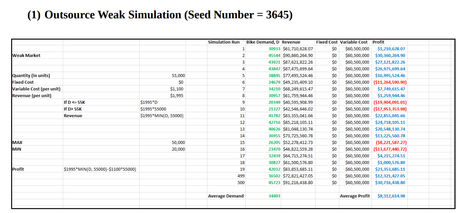
Using simulation, optimization, and decision trees, we can collect and evaluate data to make more informed business decisions. By using simulation techniques, we can better estimate model inputs subject to variability. Decision trees allow representation of the analysis while optimization will allow for figure optimal quantities. The case study presents us with several pieces of information on a company, FlowRide, an advanced commuter scooters Platform selling high-performance long-range scooters. The company is faced with a decision on whether to continue to outsource or manufacture the exercise bikes in-house. If the company decides to outsource to Hong Kong, FlowRide must purchase a minimum of 45,000 units at a cost of $875per unit with a $0 fixed cost. If they decide to manufacture the bikes in a facility in Malaysia, there is a fixed cost of $14 million with a unit cost of $685. FlowRide prices their bicycles at $1,395. We are presented with weak and strong demand scenarios with probabilities of 40% and 60% respectively. If demand is strong, the number of bikes is uniformly distributed between 35K to 65K. If the demand is weak, the number of bikes is uniformly distributed between 10K and 540K. If they outsource and the demand is greater than 45,000, they can only sell that amount. If FlowRide manufactures the bikes, they can produce an initial 25K and have the option to produce up to an additional 40K units.

Before performing the simulations, we organized all the data on cost, revenue and probability estimates in a table and then set up a decision tree with algebraic formulations to help us solve the tree once we run the simulations. Using Microsoft Excel, we simulated to estimate the expected profit using both weak and strong scenarios for outsourcing and manufacturing, we have four simulation scenarios using 500 samples each. We used the random number generator, setting it to one variable, 500 instances, uniformly with the indicated parameters. For the manufacturing scenarios, we used optimization to determine the optimal demand quantity. We used the average profit and placed it into the decision tree for each of the four scenarios and solved it accordingly. We used 3703 as our random seed. From solving the decision tree, we can determine if outsourcing or manufacturing is most profitable. Upon selecting the best scenario, we can then move forward with our recommendations to FlowRide.

Use simulation to estimate the expected profit generated for each option under both weak and strong demand scenarios. HINT: for the simulations, use 500 samples each. You will have four worksheets with simulations OUTSOURCE-WEAK; OUTSOURCE-STRONG; MANUFACTURE-WEAK; MANUFACTURE-STRONG) For the manufacturing option, use Optimization to calculate the optimal number of electric scooters to produce for both the weak and strong demand scenarios.

PLEASE SHOW THE CALCULATIONS or FORMULAS OF SIMULATION

An example of simulation is as follow:

(1) Outsource Weak Simulation (Seed Number = 3645) = Weak Market $0 Quantity (in units) Fixed Cost Variable Cost (per unit) Revenue (per unit) 55,000 $0 $1,100 $1,995 $1995*D $1995*55000 $1995*MIN(D, 55000) $0 If D 55K D Revenue Simulation Run Bike Demand, D Revenue 1 30933 $61,710,628.07 2 45544 $90,860,264.90 3 43921 $87,621,822.26 4 43847 $87,475,699.64 5 38845 $77,495,524.46 6 24679 $49,235,409.10 7 34210 $68,249,615.47 8 30957 $61,759,944.46 9 20349 $40,595,908.99 10 21327 $42,546,646.02 11 41782 $83,355,041.66 12 42716 $85,218,105.11 13 40626 $81,048,130.74 14 36955 $73,725,560.78 15 26205 $52,278,412.73 16 23470 $46,822,559.28 17 32439 $64,715,274.51 18 30827 $61,500,576.80 19 42032 $83,853,685.11 499 36502 $72,821,427.05 500 45723 $91,216,438.80 Fixed Cost Variable Cost Profit $0 $ $60,500,000 $1,210,628.07 $60,500,000 $30,360,264.90 $0 $0 $60,500,000 $27,121,822.26 $0 $60,500,000 $26,975,699.64 $0 $60,500,000 $16,995,524.46 $0 $60,500,000 ($11,264,590.90) $ $0 $60,500,000 $7,749,615.47 $0 $60,500,000 $1,259,944.46 $60,500,000 ($19,904,091.01) 0 $0 $60,500,000 ($17,953,353.98) $0 $60,500,000 $22,855,041.66 $0 $0 $60,500,000 $24,718,105.11 $0 $0 $60,500,000 $20,548,130.74 $O $0 $60,500,000 $13,225,560.78 $0 $60,500,000 ($8,221,587.27) $0 $0 $60,500,000 ($13,677,440.72) $0 $60,500,000 $4,215,274.51 $0 $60,500,000 $1,000,576.80 $0 $60,500,000 $23,353,685.11 $0 $60,500,000 $12,321,427.05 $0 $60,500,000 $30,716,438.80 MAX IMIN 50,000 20,000 Profit $1995*MIN(D, 55000) $1100*55000) Average Demand 34493 Average Profit $8,312,614.98 (1) Outsource Weak Simulation (Seed Number = 3645) = Weak Market $0 Quantity (in units) Fixed Cost Variable Cost (per unit) Revenue (per unit) 55,000 $0 $1,100 $1,995 $1995*D $1995*55000 $1995*MIN(D, 55000) $0 If D 55K D Revenue Simulation Run Bike Demand, D Revenue 1 30933 $61,710,628.07 2 45544 $90,860,264.90 3 43921 $87,621,822.26 4 43847 $87,475,699.64 5 38845 $77,495,524.46 6 24679 $49,235,409.10 7 34210 $68,249,615.47 8 30957 $61,759,944.46 9 20349 $40,595,908.99 10 21327 $42,546,646.02 11 41782 $83,355,041.66 12 42716 $85,218,105.11 13 40626 $81,048,130.74 14 36955 $73,725,560.78 15 26205 $52,278,412.73 16 23470 $46,822,559.28 17 32439 $64,715,274.51 18 30827 $61,500,576.80 19 42032 $83,853,685.11 499 36502 $72,821,427.05 500 45723 $91,216,438.80 Fixed Cost Variable Cost Profit $0 $ $60,500,000 $1,210,628.07 $60,500,000 $30,360,264.90 $0 $0 $60,500,000 $27,121,822.26 $0 $60,500,000 $26,975,699.64 $0 $60,500,000 $16,995,524.46 $0 $60,500,000 ($11,264,590.90) $ $0 $60,500,000 $7,749,615.47 $0 $60,500,000 $1,259,944.46 $60,500,000 ($19,904,091.01) 0 $0 $60,500,000 ($17,953,353.98) $0 $60,500,000 $22,855,041.66 $0 $0 $60,500,000 $24,718,105.11 $0 $0 $60,500,000 $20,548,130.74 $O $0 $60,500,000 $13,225,560.78 $0 $60,500,000 ($8,221,587.27) $0 $0 $60,500,000 ($13,677,440.72) $0 $60,500,000 $4,215,274.51 $0 $60,500,000 $1,000,576.80 $0 $60,500,000 $23,353,685.11 $0 $60,500,000 $12,321,427.05 $0 $60,500,000 $30,716,438.80 MAX IMIN 50,000 20,000 Profit $1995*MIN(D, 55000) $1100*55000) Average Demand 34493 Average Profit $8,312,614.98