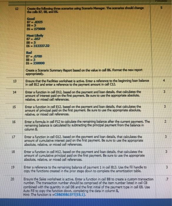
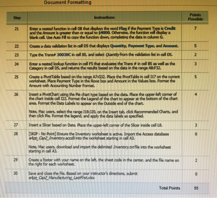
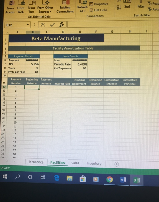
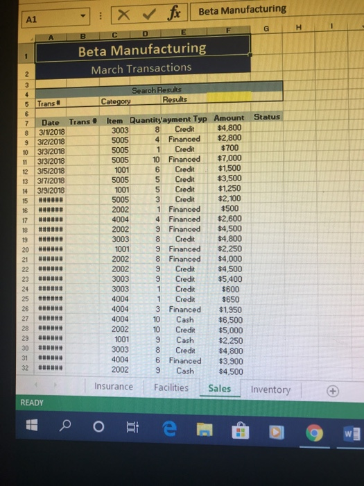
using the excell sheets as refrence i need questions 11-30 solved using pictures to describe each step. let me know if more information is needed.

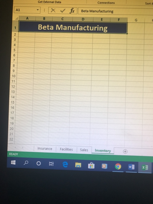
can we just work around this for the sake of time. the other answers will be more important... thank you.

dont worry about it. i got the questions answered

11 Ensure that the Facilities worksheet is active. Use Goal Seek to reduce the monthly payment in cell B6 to the optimal value of $6000. Complete this task by changing the Loan amount in cell E6. 12 Create the following three scenarios using Scenario Manager. The scenarios should change the cels B7, B8, and E6. Good B7 = .0325 B85 56 = 275000 Most likely B7 = .057 B8 = 5 E6 =31222732 Bad B7 = .0700 B8 = 3 E6 = 350000 Create a Scenario Summary Report based on the value in cell B6. Format the new report appropriately. Ensure that the Facilities worksheet is active. Enter a reference to the beginning loan balance in cell B12 and enter a reference to the payment amount in cel C12 13 16 Enter a function in oall D12, based on the payment and loan details, that calculates the amount of interest paid on the first payment. Be sure to use the appropriate absolute. relative, or mored cell references. Enter a function in cell E12, based on the payment and loan details, that calculates the amount of principal paid on the first payment. Be sure to use the appropriate absolute, relative, or mored cell references. Enter a formula in cell F12 to calculate the remaining balance after the current payment. The remaining balance is calculated by subtracting the principal payment from the balance in column B Enter a function in cell G12, based on the payment and loan details, that calculates the amount of cumulative interest paid on the first payment. Be sure to use the appropriate absolute, relative, or mixed cell references. Enter a function in cell H12, based on the payment and loan details, that calculates the amount of cumulative principal paid on the first payment. Be sure to use the appropriate absolute, relative, or moved cell references. 17 Enter a reference to the remaining balance of payment 1 in cel B13. Use the fill hande to copy the functions created in the prior steps down to complete the amortization table. 7 Ensure the sales worksheet is active. Enter a function in cel B8 to create a custom transaction number. The transaction number should be comprised of the item number listed in cel C8 combined with the quantity in cel Ds and the first initial of the payment type in cell E8. Use Auto Fill to copy the function down, completing the data in column B Hint: The function is =C88DLEFT(E8,1). Document Formatting Step Instructions Points Possible NIN 26 Enter a nested function in cell G8 that displays the word Flag if the Payment Type is Credit and the Amount is greater than or equal to $4000. Otherwise, the function will display a blank call. Use Auto Fill to copy the function down, completing the data in column G. Create a data validation list in cell DS that displays Quantity, Payment Type, and Amor Type the Trans# 30038C in cell BS, and select Quantity from the validation list in cell DS. Enter a nested lookup function in call 5 that evaluates the Trans # in cell B5 as well as the Category in cell D5, and returns the results based on the data in the range AB:F32. Create a Pivot Table based on the range A7:G32. Place the Pivot Table in cell 117 on the current worksheet. Place Payment Type in the Rows box and Amount in the Values box. Format the Amount with Accounting Number Format. Insert a PivotChart using the Pie chart type based on the data. Place the upper-left comer of the chart inside cell 122. Format the Legend of the chart to appear at the bottom of the chart area. Format the Data Labels to appear on the Outside end of the chart. Note, Mac users, select the range [18:320, on the Insert tab, dick Recommended Charts, and then dick Pie Format the legend, and apply the data labels as specified. Insert a Slicer based on Date. Place the upper-left corner of the Slicer inside cell 18. (SKIP - No Point) Ensure the Inventory worksheet is active. Import the Access database 24g_app Inventory.accabinto the worksheet starting in cel A3. Note, Mac users, download and import the delimited Inventory.bit file into the worksheet starting in cell A3. Create a footer with your name on the left, the sheet code in the center, and the file name on the right for each worksheet. Save and close the file. Based on your instructor's directions, submit e4pp_Cap2 Manufacturing LastFirstads Total Points 2- AZ 1 Sort Filter From From Access Web Rear To Advi Sort & Filter 26 E L S Properties From From Other Existing Refresh Text Sources Connections All - Edit Links Get External Data Connections : X for B C D E F Beta Manufacturing B12 I A G AN Facility Amortization Table Payment Details 6 Payment 7 APR 5.7596 8 Years 9 Pmts per Year 12 Loan Details Loan Periodic Rate 0.479% # of Payments 60 Payment Number Beginning Payment Principal Balance Amount Interest Paid Repayment Remaining Cumulative Balance Interest Cumulative Principal Insurance Facilities Sales Inventory + READY o 20 te gwixi - : x fr Beta Manufacturing Beta Manufacturing March Transactions Search Results Category Results on Trans c 11 12 Date 3/12018 3/2/2018 3/3/2018 3/3/2018 315/2018 317/2018 3/9/2018 ### ### ## ### ## # Trans. Item Quantity'ayment Typ Amount Status 3003 8 Credit $4,800 5005 4 Financed $2,800 5005 1 Credit $700 5005 10 Financed 1001 6 Credit $1,500 5005 5 Credit $3,500 1001 5 Credit $1,250 5005 3 Credit $2,100 2002 1 Financed $500 4004 4 Financed $2,600 2002 9 Financed $4,500 3003 8 Credit $4,800 1001 9 Financed $2,250 2002 8 Financed $4,000 2002 9 Credit $4,500 3003 9 Credit $5,400 3003 1 Credit $600 4004 1 Credit $650 4004 3 Financed $1,950 4004 10 Cash $6,500 2002 10 Credit $5,000 1001 9 Cash $2,250 3003 8 Credit $4,800 4004 6 Financed $3,900 2002 9 Cash $4,500 Insurance Facilities Sales Inventory READY 1. OBI em D9wg Get External Data Connections Sorte A X fx Beta Manufacturing B C D E Beta Manufacturing F Insurance Facilities Sales Inventory + READY 11 Ensure that the Facilities worksheet is active. Use Goal Seek to reduce the monthly payment in cell B6 to the optimal value of $6000. Complete this task by changing the Loan amount in cell E6. 12 Create the following three scenarios using Scenario Manager. The scenarios should change the cels B7, B8, and E6. Good B7 = .0325 B85 56 = 275000 Most likely B7 = .057 B8 = 5 E6 =31222732 Bad B7 = .0700 B8 = 3 E6 = 350000 Create a Scenario Summary Report based on the value in cell B6. Format the new report appropriately. Ensure that the Facilities worksheet is active. Enter a reference to the beginning loan balance in cell B12 and enter a reference to the payment amount in cel C12 13 16 Enter a function in oall D12, based on the payment and loan details, that calculates the amount of interest paid on the first payment. Be sure to use the appropriate absolute. relative, or mored cell references. Enter a function in cell E12, based on the payment and loan details, that calculates the amount of principal paid on the first payment. Be sure to use the appropriate absolute, relative, or mored cell references. Enter a formula in cell F12 to calculate the remaining balance after the current payment. The remaining balance is calculated by subtracting the principal payment from the balance in column B Enter a function in cell G12, based on the payment and loan details, that calculates the amount of cumulative interest paid on the first payment. Be sure to use the appropriate absolute, relative, or mixed cell references. Enter a function in cell H12, based on the payment and loan details, that calculates the amount of cumulative principal paid on the first payment. Be sure to use the appropriate absolute, relative, or moved cell references. 17 Enter a reference to the remaining balance of payment 1 in cel B13. Use the fill hande to copy the functions created in the prior steps down to complete the amortization table. 7 Ensure the sales worksheet is active. Enter a function in cel B8 to create a custom transaction number. The transaction number should be comprised of the item number listed in cel C8 combined with the quantity in cel Ds and the first initial of the payment type in cell E8. Use Auto Fill to copy the function down, completing the data in column B Hint: The function is =C88DLEFT(E8,1). Document Formatting Step Instructions Points Possible NIN 26 Enter a nested function in cell G8 that displays the word Flag if the Payment Type is Credit and the Amount is greater than or equal to $4000. Otherwise, the function will display a blank call. Use Auto Fill to copy the function down, completing the data in column G. Create a data validation list in cell DS that displays Quantity, Payment Type, and Amor Type the Trans# 30038C in cell BS, and select Quantity from the validation list in cell DS. Enter a nested lookup function in call 5 that evaluates the Trans # in cell B5 as well as the Category in cell D5, and returns the results based on the data in the range AB:F32. Create a Pivot Table based on the range A7:G32. Place the Pivot Table in cell 117 on the current worksheet. Place Payment Type in the Rows box and Amount in the Values box. Format the Amount with Accounting Number Format. Insert a PivotChart using the Pie chart type based on the data. Place the upper-left comer of the chart inside cell 122. Format the Legend of the chart to appear at the bottom of the chart area. Format the Data Labels to appear on the Outside end of the chart. Note, Mac users, select the range [18:320, on the Insert tab, dick Recommended Charts, and then dick Pie Format the legend, and apply the data labels as specified. Insert a Slicer based on Date. Place the upper-left corner of the Slicer inside cell 18. (SKIP - No Point) Ensure the Inventory worksheet is active. Import the Access database 24g_app Inventory.accabinto the worksheet starting in cel A3. Note, Mac users, download and import the delimited Inventory.bit file into the worksheet starting in cell A3. Create a footer with your name on the left, the sheet code in the center, and the file name on the right for each worksheet. Save and close the file. Based on your instructor's directions, submit e4pp_Cap2 Manufacturing LastFirstads Total Points 2- AZ 1 Sort Filter From From Access Web Rear To Advi Sort & Filter 26 E L S Properties From From Other Existing Refresh Text Sources Connections All - Edit Links Get External Data Connections : X for B C D E F Beta Manufacturing B12 I A G AN Facility Amortization Table Payment Details 6 Payment 7 APR 5.7596 8 Years 9 Pmts per Year 12 Loan Details Loan Periodic Rate 0.479% # of Payments 60 Payment Number Beginning Payment Principal Balance Amount Interest Paid Repayment Remaining Cumulative Balance Interest Cumulative Principal Insurance Facilities Sales Inventory + READY o 20 te gwixi - : x fr Beta Manufacturing Beta Manufacturing March Transactions Search Results Category Results on Trans c 11 12 Date 3/12018 3/2/2018 3/3/2018 3/3/2018 315/2018 317/2018 3/9/2018 ### ### ## ### ## # Trans. Item Quantity'ayment Typ Amount Status 3003 8 Credit $4,800 5005 4 Financed $2,800 5005 1 Credit $700 5005 10 Financed 1001 6 Credit $1,500 5005 5 Credit $3,500 1001 5 Credit $1,250 5005 3 Credit $2,100 2002 1 Financed $500 4004 4 Financed $2,600 2002 9 Financed $4,500 3003 8 Credit $4,800 1001 9 Financed $2,250 2002 8 Financed $4,000 2002 9 Credit $4,500 3003 9 Credit $5,400 3003 1 Credit $600 4004 1 Credit $650 4004 3 Financed $1,950 4004 10 Cash $6,500 2002 10 Credit $5,000 1001 9 Cash $2,250 3003 8 Credit $4,800 4004 6 Financed $3,900 2002 9 Cash $4,500 Insurance Facilities Sales Inventory READY 1. OBI em D9wg Get External Data Connections Sorte A X fx Beta Manufacturing B C D E Beta Manufacturing F Insurance Facilities Sales Inventory + READY