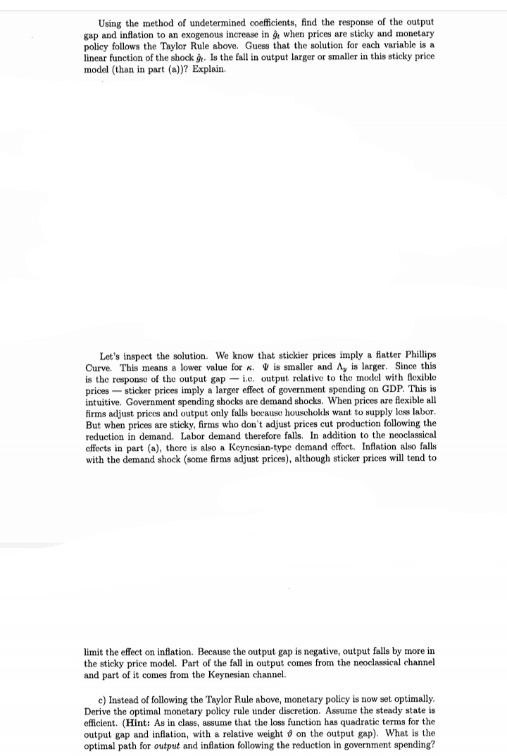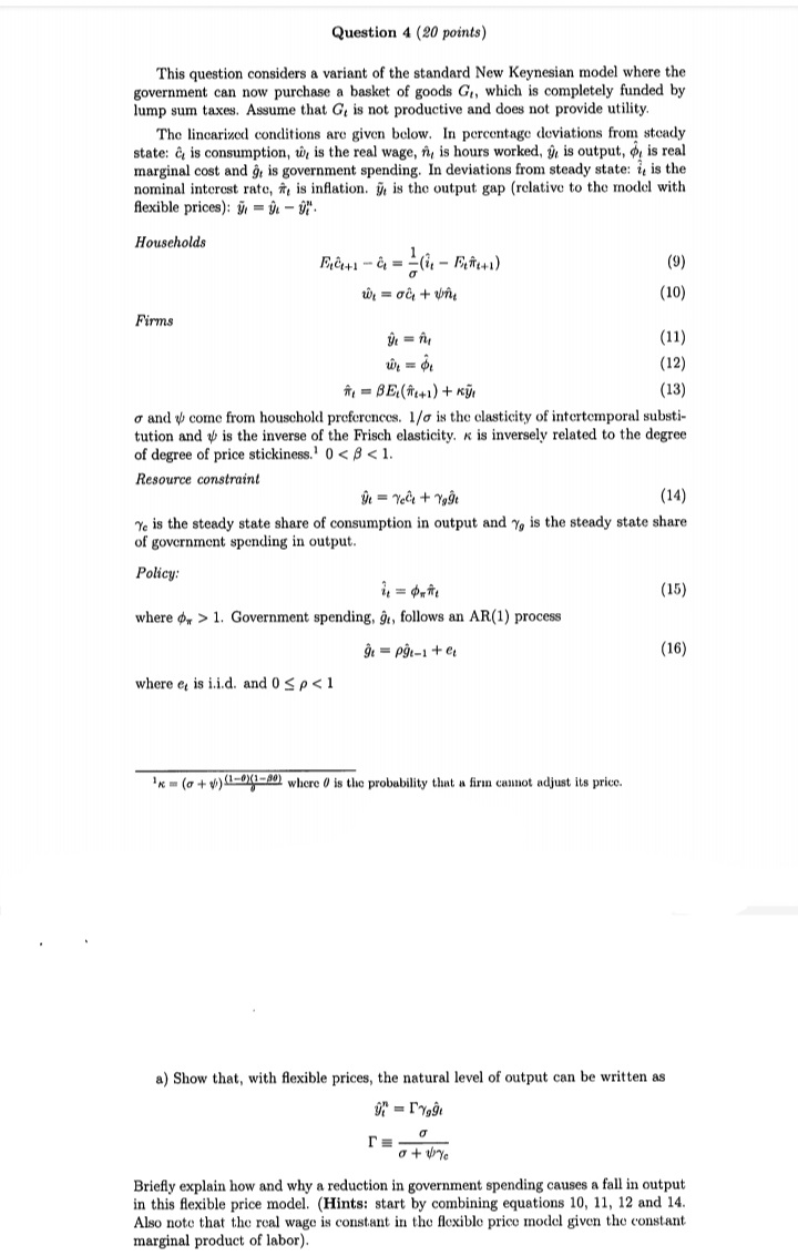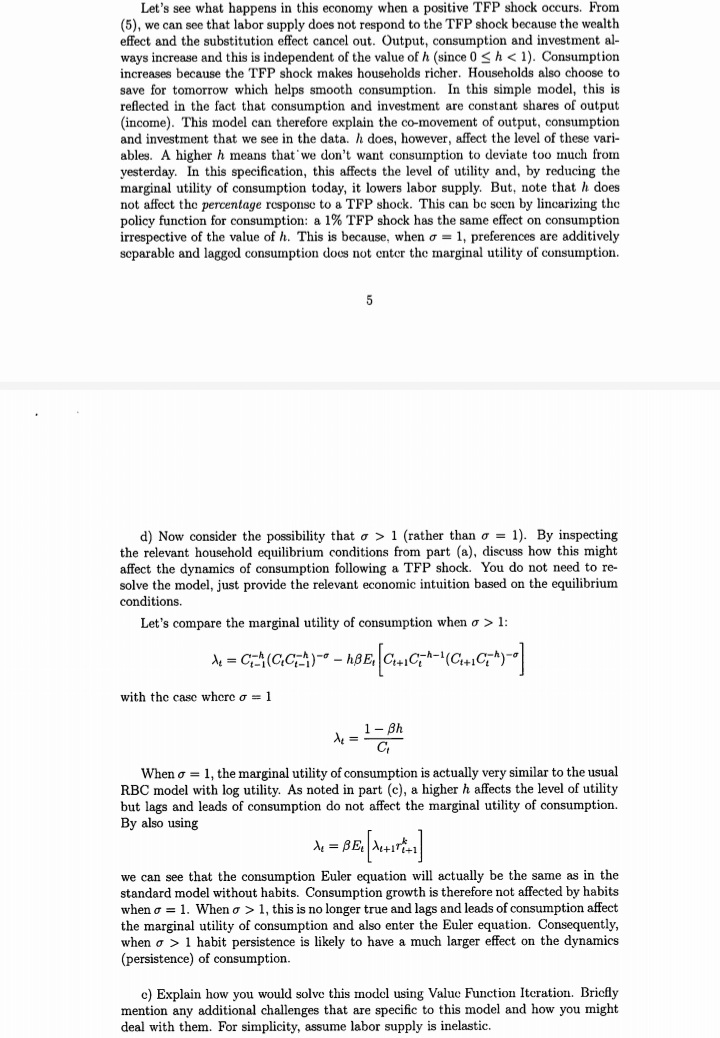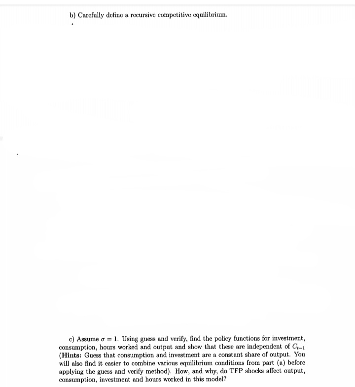
Using the method of undetermined coefficients, find the response of the output gap and inflation to an exogenous increase in g, when prices are sticky and monetary policy follows the Taylor Rule above. Guess that the solution for each variable is a linear function of the shock g. Is the fall in output larger or smaller in this sticky price model (than in part (a))? Explain. Let's inspect the solution. We know that stickier prices imply a flatter Phillips Curve. This means a lower value for a. I is smaller and A, is larger. Since this is the response of the output gap - i.c. output relative to the model with flexible prices - sticker prices imply a larger effect of government spending on GDP. This is intuitive. Government spending shocks are demand shocks. When prices are flexible all firms adjust prices and output only falls because households want to supply less labor. But when prices are sticky, firms who don't adjust prices cut production following the reduction in demand. Labor demand therefore falls. In addition to the neoclassical effects in part (a), there is also a Keynesian-type demand effect. Inflation also falls with the demand shock (some firms adjust prices), although sticker prices will tend to limit the effect on inflation. Because the output gap is negative, output falls by more in the sticky price model. Part of the fall in output comes from the neoclassical channel and part of it comes from the Keynesian channel c) Instead of following the Taylor Rule above, monetary policy is now set optimally. Derive the optimal monetary policy rule under discretion. Assume the steady state is efficient. (Hint: As in class, assume that the loss function has quadratic terms for the output gap and inflation, with a relative weight of on the output gap). What is the optimal path for output and inflation following the reduction in government spending?Question 4 (20 points) This question considers a variant of the standard New Keynesian model where the government can now purchase a basket of goods Gr, which is completely funded by lump sum taxes. Assume that G, is not productive and does not provide utility. The lincarized conditions are given below. In percentage deviations from steady state: & is consumption, w, is the real wage, n, is hours worked, y, is output, o, is real marginal cost and g, is government spending. In deviations from steady state: i, is the nominal interest rate, #, is inflation. # is the output gap (relative to the model with flexible prices): y, = it - Up. Households (9) (10) Firms (11) (12) it = BE (1 +1) + ky (13) o and of come from household preferences. 1/ is the clasticity of intertemporal substi tution and v is the inverse of the Frisch elasticity. 1. Government spending, gr, follows an AR(1) process go = pgi-1 + et (16) where er is i.i.d. and 0 S p 1 (rather than o = 1). By inspecting the relevant household equilibrium conditions from part (a), discuss how this might affect the dynamics of consumption following a TFP shock. You do not need to re- solve the model, just provide the relevant economic intuition based on the equilibrium conditions. Let's compare the marginal utility of consumption when o > 1: M = C(CC)- - BE, CHICT-(CHICTA)-] with the case where o = 1 de = 1 - Bh C When o = 1, the marginal utility of consumption is actually very similar to the usual RBC model with log utility. As noted in part (c), a higher h affects the level of utility but lags and leads of consumption do not affect the marginal utility of consumption. By also using we can see that the consumption Euler equation will actually be the same as in the standard model without habits. Consumption growth is therefore not affected by habits when o = 1. When o > 1, this is no longer true and lags and leads of consumption affect the marginal utility of consumption and also enter the Euler equation. Consequently, when o > 1 habit persistence is likely to have a much larger effect on the dynamics (persistence) of consumption. c) Explain how you would solve this model using Value Function Iteration. Briefly mention any additional challenges that are specific to this model and how you might deal with them. For simplicity, assume labor supply is inelastic.b) Carefully define a recursive competitive equilibrium. c) Assume