vicsek2d matlab code:

function gobs=vicsek2d(N, ts, eta, top, topval, gobsFlag, boundary, show)

% function X=vicsek2d(N, ts, eta, rad, show)

%

% eta is the the noise value for dtheta

% ts number of timesteps

% N is the number of birds

% top is the topology ('metric', 'nn')

% topval is the value for metric, radius, for nn number of nearest

% neighbors

% gobsFlag is 1 for computing global observables and 0 for not

% boundary is 0 for periodic and 1 for reflective

% show is 1 if you want to plot. set to 0 for analysis

%

% Vicsek, T., Czirak, A., Ben-Jacob, E., Cohen, I., & Shochet, O. (1995).

% Novel Type of Phase Transition in a System of Self-Driven Particles.

% Physical Review Letters, 75, 1226-1229. doi:10.1103/PhysRevLett.75.1226

% s = RandStream('mt19937ar','Seed',1);

% RandStream.setGlobalStream(s);

% default params if you run it as is

if nargin ==0

N=400; ts=500; eta=pi/6; top='metric'; topval=2; show=1;

gobsFlag=0;

boundary=2; % 0=periodic, 1=reflective, 2=circular

end

gobs.annd=zeros(1,ts);

gobs.pol=zeros(1,ts);

gobs.angm=zeros(1,ts);

gk=ts-min(ts/10, 40);

% note that we assign units but these could be anything to match whatever

% is realistic

b=[-5 5 -5 5]; % boundary (m)

sp=.03; % speed m/s

dt=1; % seconds?

% initialize

x1=zeros(N,ts); x2=x1; v1=x1; v2=x1;

% use component-wise to speed up code

x1(:,1)=b(1)+rand(N,1)*(b(2)-b(1)); % x_1

x2(:,1)=b(3)+rand(N,1)*(b(4)-b(3)); % x_2

if boundary==2

% note that this may not be the correct way to sample uniformly within

% a circle, but we will approx. since it should not affect our final

% results.

thk=rand(N,1)*2*pi;

x1(:,1)=(b(2)-b(1))/2*rand(N,1).*cos(thk);

x2(:,1)=(b(2)-b(1))/2*rand(N,1).*sin(thk);

end

v1(:,1)=randn(N,1); % xdot_1 / v_1 (direction only)

v2(:,1)=randn(N,1); % xdot_2 / v_2 (direction only)

for k=1:ts

% topology

D=sqrt((x1(:,k)*ones(1,N)-ones(N,1)*x1(:,k)').^2 + ...

(x2(:,k)*ones(1,N)-ones(N,1)*x2(:,k)').^2);

% motion model | equation (1) in paper

x1(:,k+1)=x1(:,k)+sp*v1(:,k)*dt;

x2(:,k+1)=x2(:,k)+sp*v2(:,k)*dt;

for ii=1:N

% interaction rule

% metric

if strcmp(top, 'metric')

rad=topval;

nidx=find(D(ii,:)

elseif strcmp(top, 'nn')

% or n nearest neighbors

nn=topval;

[~, nidx]=sort(D(ii,:));

nidx=nidx(1:nn); % including ii

end

% average angle

sin_th=sum(v2(nidx,k))umel(nidx);

cos_th=sum(v1(nidx,k))umel(nidx);

if ~isempty(nidx)

th_hat_ri=atan2(sin_th, cos_th);

else

th_hat_ri=0;

end

% direction update | equation (2) in paper

th=th_hat_ri-eta/2 + rand*eta;

% update the direction for the next time-step

v1(ii,k+1)=cos(th);

v2(ii,k+1)=sin(th);

end

if boundary==0

% periodic boundary condition

x1(x1(:,k+1)

x1(x1(:,k+1)>b(2),k+1)=x1(x1(:,k+1)>b(2),k+1)-(b(2)-b(1));

x2(x2(:,k+1)

x2(x2(:,k+1)>b(4),k+1)=x2(x2(:,k+1)>b(4),k+1)-(b(4)-b(3));

elseif boundary==1

% reflective boundary condition

v1(x1(:,k+1)

x1(x1(:,k+1)

v1(x1(:,k+1)>b(2),k+1)=-v1(x1(:,k+1)>b(2),k+1);

x1(x1(:,k+1)>b(2),k+1)=x1(x1(:,k+1)>b(2),k+1)+v1(x1(:,k+1)>b(2),k+1)*sp;

v2(x2(:,k+1)

x2(x2(:,k+1)

v2(x2(:,k+1)>b(4),k+1)=-v2(x2(:,k+1)>b(4),k+1);

x2(x2(:,k+1)>b(4),k+1)=x2(x2(:,k+1)>b(4),k+1)+v2(x2(:,k+1)>b(4),k+1)*sp;

elseif boundary==2

% reflective circular boundary

rk=sqrt(x1(:,k+1).^2+x2(:,k+1).^2);

ct=x1(:,k+1)./rk;

st=x2(:,k+1)./rk;

outidx=(rk>(b(2)-b(1))/2);

if sum(outidx)

% v=vt+vn

% v'=vt-vn=vt+vn-2*vn=v-2*vn;

% vn1=x1*v1/rk

vn=v1(:,k+1).*ct+v2(:,k+1).*st;

v1(outidx,k+1)=v1(outidx,k+1)-2*ct(outidx).*vn(outidx);

v2(outidx,k+1)=v2(outidx,k+1)-2*st(outidx).*vn(outidx);

nv=sqrt(v1(outidx,k+1).^2+v2(outidx,k+1).^2);

v1(outidx,k+1)=v1(outidx,k+1).v;

v2(outidx,k+1)=v2(outidx,k+1).v;

x1(outidx, k+1)=x1(outidx, k+1)+v1(outidx,k+1)*sp;

x2(outidx, k+1)=x2(outidx, k+1)+v2(outidx,k+1)*sp;

end

end

if gobsFlag

% only compute for the last tenth of the time

if k > gk

gobs.annd(1,k)=annd(D);

gobs.pol(1,k)=pol([v1(:,k)'; v2(:,k)']);

gobs.angm(1,k)=ang_m([v1(:,k)'; v2(:,k)'], [x1(:,k)'; x2(:,k)']);

else

gobs.annd(1,k)=nan;

gobs.pol(1,k)=nan;

gobs.angm(1,k)=nan;

end

end

% display; alternatively use the output for analysis

if show

figure(1); gcf;

if gobsFlag

subplot(2,2,1); gca; cla;

else

clf;

end

plot(x1(:,k), x2(:,k), 'b.');

hold on;

axis(b);

axis square;

quiver(x1(:,k), x2(:,k), v1(:,k)*.25, v2(:,k)*.25, 0, 'k');

xlabel(sprintf('[%d]', k));

if boundary==2

th=linspace(-pi, pi, 50);

plot((b(2)-b(1))/2*cos(th), (b(2)-b(1))/2*sin(th), 'b');

end

if gobsFlag

% annd

subplot(2,2,2); gca; cla;

plot(1:k, gobs.annd(1,1:k), 'linewidth', 2);

hold on;

xlabel('time'); ylabel('annd (m)');

axis([0 ts 0 (b(2)-b(1))/2]);

% pol

subplot(2,2,3); gca; cla;

plot(1:k, gobs.pol(1,1:k), 'linewidth', 2);

hold on;

xlabel('time'); ylabel('pol');

axis([0 ts 0 1]);

% angular momentum

subplot(2,2,4); gca; cla;

plot(1:k, gobs.angm(1,1:k), 'linewidth', 2);

hold on;

xlabel('time'); ylabel('normalized angular momentum');

axis([0 ts 0 1]);

end

drawnow;

end

end

function [dat, perm]=annd(D)

% function annd(r)

% average nearest-neighbor distance

%

% r is a d x n matrix with d dimensions and n targets

D=D+eye(size(D,1))*100000000;

[perm, ~]=min(D);

dat=mean(perm);

function P=pol(v)

% function pol(v)

%

% v is a d x n matrix with d dimensions and n targets

[d, n]=size(v);

vhat = v./(ones(d,1)*sqrt(sum(v.^2)));

P=1*norm(sum(vhat,2));

function am=ang_m(v,rf)

[d, n]=size(v);

vhat = v./(ones(d,1)*sqrt(sum(v.^2)));

rf=rf-mean(rf,2)*ones(1,size(rf,2));

if size(rf,2) == size(v,2)

rf=[rf; zeros(1,size(rf,2))];

vhat=[vhat; zeros(1,size(vhat,2))];

am=norm(sum(cross(rf,vhat),2))/sum(sqrt(sum(rf.^2)).*sqrt(sum(vhat.^2)));

% am=dot(sum(cross(rf,vhat),2), [0 0 1]')/sum(sqrt(sum(cross(rf,vhat).^2,1)));

% am=dot(sum(cross(rf,vhat),2), [0 0 1]')/sum(sqrt(sum(rf.^2)).*sqrt(sum(vhat.^2)));

% am=norm(dot(sum(cross(rf,vhat),2), [0 0 1]'));

% am=dot(sum(cross(rf,vhat),2), [0 0 1]');

% am=norm(dot(sum(cross(rf,vhat),2), [0 0 1]'));

else

am=nan;

end

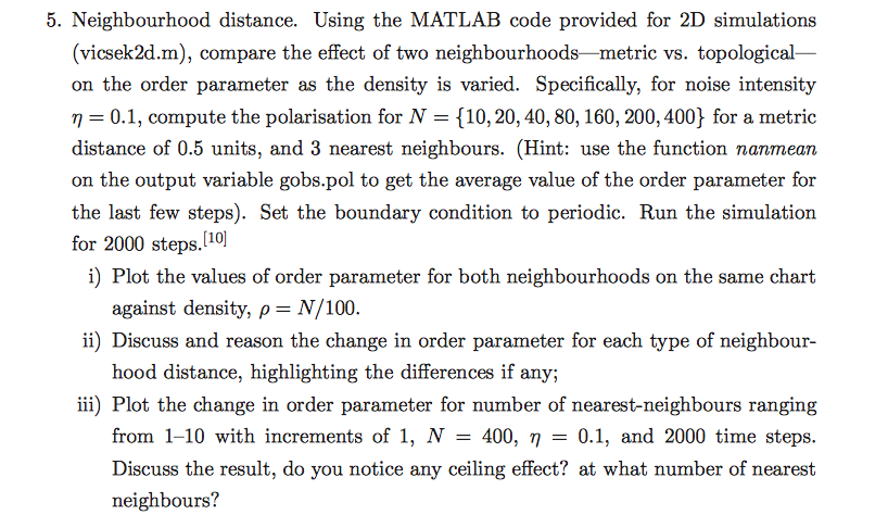
5. Neighbourhood distance. Using the MATLAB code provided for 2D simulations (vicsek2d.m), compare the effect of two neighbourhoods metric vs. topological on the order parameter as the density is varied. Specifically, for noise intensity = 0.1, compute the polarisation for N = {10, 20, 40, 80, 160, 200, 400} for a metric distance of 0.5 units, and 3 nearest neighbours. (Hint: use the function nanmean on the output variable gobs.pol to get the average value of the order parameter for the last few steps). Set the boundary condition to periodic. Run the simulation for 2000 steps. [I i) Plot the values of order parameter for both neighbourhoods on the same chart ii) Discuss and reason the change in order parameter for each type of neighbour- ) Plot the change in order parameter for number of nearest-neighbours ranging 400, = 0.1, and 2000 time steps. Discuss the result, do you notice any ceiling effect? at what number of nearest hood distance, highlighting the differences if any; from 1-10 with increments of 1, N neighbours? 5. Neighbourhood distance. Using the MATLAB code provided for 2D simulations (vicsek2d.m), compare the effect of two neighbourhoods metric vs. topological on the order parameter as the density is varied. Specifically, for noise intensity = 0.1, compute the polarisation for N = {10, 20, 40, 80, 160, 200, 400} for a metric distance of 0.5 units, and 3 nearest neighbours. (Hint: use the function nanmean on the output variable gobs.pol to get the average value of the order parameter for the last few steps). Set the boundary condition to periodic. Run the simulation for 2000 steps. [I i) Plot the values of order parameter for both neighbourhoods on the same chart ii) Discuss and reason the change in order parameter for each type of neighbour- ) Plot the change in order parameter for number of nearest-neighbours ranging 400, = 0.1, and 2000 time steps. Discuss the result, do you notice any ceiling effect? at what number of nearest hood distance, highlighting the differences if any; from 1-10 with increments of 1, N neighbours