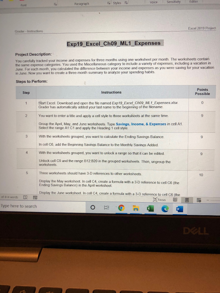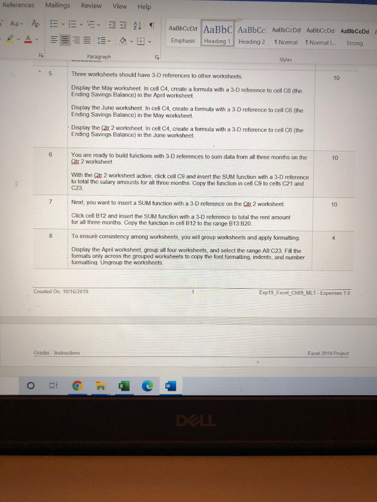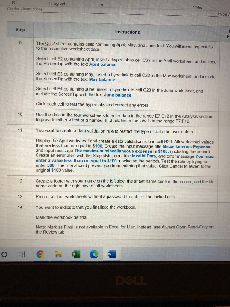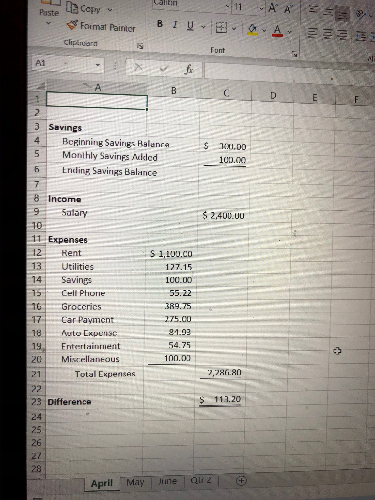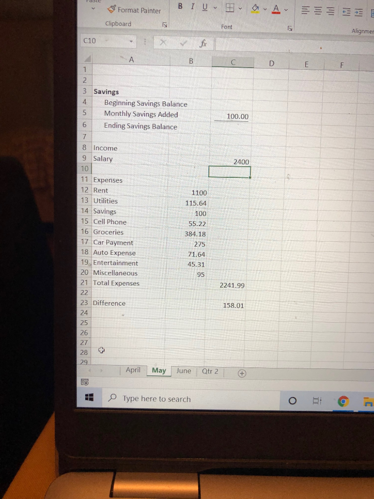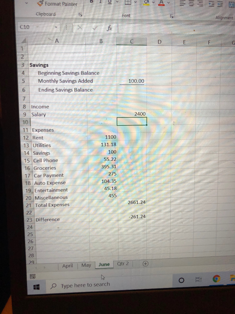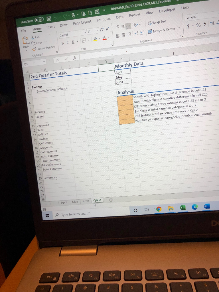
Voice Sensitivity Editor Styles 5 Font Paragraph Excel 2019 Project Grader - Instructions Exp19_Excel_Ch09_ML1_Expenses Project Description: You carefully tracked your income and expenses for three months using one worksheet per month. The worksheets contain the same expense categories. You used the Miscellaneous category to include a variety of expenses, including a vacation in June. For each month, you calculated the difference between your income and expenses as you were saving for your vacation in June. Now you want to create a three-month summary to analyze your spending habits. Steps to Perform: Step Instructions Points Possible 1 0 Start Excel. Download and open the file named Exp19_Excel_Ch09 ML1_Expenses xlsx Grader has automatically added your last name to the beginning of the filename. 2 9 You want to enter a title and apply a cell style to three worksheets at the same time. Group the April, May, and June worksheets. Type Savings, Income, & Expenses in cell A1. Select the range A1 C1 and apply the Heading 1 cell style. With the worksheets grouped, you want to calculate the Ending Savings Balance 3 9 In cell C6, add the Beginning Savings Balance to the Monthly Savings Added. 4 9 With the worksheets grouped, you want to unlock a range so that it can be edited. Unlock cell C9 and the range B12:B20 in the grouped worksheets. Then, ungroup the worksheets. 5 Three worksheets should have 3-D references to other worksheets 10 Display the May worksheet. In cell C4, create a formula with a 3D reference to cell C6 (the Ending Savings Balance) in the April worksheet. Display the June worksheet. In cell C4, create a formula with a 3-D reference to cell C6 (the EO Focus of 814 words DS Type here to search DELL References Mailings Review View Help a Aa- A E E 21 T AaBbCcDd AaBbc AaBbCc AaBbCcDdl AaBbCcDd AaBbCcDd Emphasis Heading 1 Heading 2 1 Normal 1 Normal ... Strong Paragraph www Styles 5 Three worksheets should have 3-D references to other worksheets 10 Display the May worksheet. In cell C4, create a formula with a 3-D reference to cell C6 (the Ending Savings Balance) in the Apnl worksheet Display the June worksheet. In cell C4, create a formula with a 3-D reference to cell C6 (the Ending Savings Balance) in the May worksheet. Display the Qir 2 worksheet. In cell C4, create a formula with a 3-D reference to cell C6 (the Ending Savings Balance) in the June worksheet 6 You are ready to build functions with 3-D references to sum data from all three months on the Qtr 2 worksheet 10 With the Qtr 2 worksheet active click cell C9 and insert the SUM function with a 3-D reference to total the salary amounts for all three months. Copy the function in cell C9 to cells C21 and C23 7 10 Next, you want to insert a SUM function with a 3-D reference on the Qir 2 worksheet Click cell B12 and insert the SUM function with a 3-D reference to total the rent amount for all three months. Copy the function in cell B12 to the range B13:B20 8 4 To ensure consistency among worksheets, you will group worksheets and apply formatting Display the April worksheet, group all four worksheets, and select the range A8 C23. Fill the formats only across the grouped worksheets to copy the font formatting, indents, and number formatting. Ungroup the worksheets Created On: 10/16/2019 Exp19 Excel_Ch09_ML1 - Expenses 1.0 Grader - Instructions Excel 2019 Project O DELL Paragraph Grader - Instructions Styles Excel Step Instructions P 9 The Qtr 2 sheet contains cells containing April, May, and June text. You will insert hyperlinks to the respective worksheet data. Select cell E2 containing April, insert a hyperlink to cell C23 in the April worksheet, and include the Screen Tip with the text April balance. Select cell E3 containing May, insert a hyperlink to cell C23 in the May worksheet, and include the Screen Tip with the text May balance. Select cell E4 containing June, insert a hyperlink to cell C23 in the June worksheet, and include the Screen Tip with the text June balance. Click each cell to test the hyperlinks and correct any errors. 10 Use the data in the four worksheets to enter data in the range E7:E12 in the Analysis section to provide either a text or a number that relates to the labels in the range F7 F12. 11 You want to create a data validation rule to restrict the type of data the user enters. Display the April worksheet and create a data validation rule in cell B20. Allow decimal values that are less than or equal to $100. Create the input message title Miscellaneous Expense and input message The maximum miscellaneous expense is $100. (including the period). Create an error alert with the Stop style, error title Invalid Data, and error message You must enter a value less than or equal to $100. (including the period). Test the rule by trying to enter 500. The rule should prevent you from entering that value. Click Cancel to revert to the original $100 value. 12 Create a footer with your name on the left side, the sheet name code in the center, and the file name code on the right side of all worksheets. 13 Protect all four worksheets without a password to enforce the locked cells. 14 You want to indicate that you finalized the workbook. Mark the workbook as final. Note: Mark as Final is not available in Excel for Mac. Instead, use Always Open Read-Only on the Review tab. DI W Calibri ~11 Paste A == LE Copy Format Painter BI UB CA V Clipboard Font A1 fr B D E F 12 C 1 2. 3 Savings 4 Beginning Savings Balance $ 300.00 5 Monthly Savings Added 100.00 6 Ending Savings Balance 7 8 Income Salary $ 2,400.00 10 11 Expenses Rent $ 1,100.00 13 Utilities 127.15 14 Savings 100.00 15 Cell Phone 55.22 16 Groceries 389.75 17 Car Payment 275.00 18 Auto Expense 84.93 19 Entertainment 54.75 20 Miscellaneous 100.00 21 Total Expenses 2,286.80 22 23 Difference S 113.20 24 25 26 27 28 May June Qtr 2 + April Format Painter BI UB a. Av Clipboard Font Alignmer C10 B C D E F 1 2 100.00 2400 3 Savings 4 Beginning Savings Balance 5 Monthly Savings Added 6 Ending Savings Balance 7 8 Income 9 Salary 10 11 Expenses 12 Rent 1100 13 Utilities 115.64 14 Savings 100 15 Cell Phone 55.22 16 Groceries 384.18 17 Car Payment 275 18 Auto Expense 71.64 19. Entertainment 45.31 20 Miscellaneous 95 21 Total Expenses 22 23 Difference 24 2241.99 158.01 25 26. 27 28 29 April May June Qtr 2 + LO Type here to search O 1 Format Painter A Clipboard Font Alignment C10 A B C D G 1 2 3 Savings 4 Beginning Savings Balance 5 Monthly Savings Added 6 Ending Savings Balance 7 100.00 8 Income 9 Salary 2400 10 11 Expenses 12 Rent 13 Utilities 14 Savings 15 Cell Phone 16 Groceries 17 Car Payment 18 Auto Expense 19 Entertainment 20 Miscellaneous 21 Total Expenses 22 23 Difference 24 25 26 27 1100 131.18 100 55.22 395.31 275 104.35 45.18 455 2661.24 -261.24 28 29 April May June Qtr 2 EO Type here to search RAHMAN_Exp 19_Excel_Ch09_ML1_Expenses Help View Developer Review Data General Formulas AutoSave OH Draw Page Layout Wrap Text Insert $ % to Home File - 11 - A 3 Merge & Center Nurnber Calibri X Cut A - BIU Alignment 15 Paste [ $ Format Painter Font F Clipboard f D p1 C B E Monthly Data April May June 1 2nd Quarter Totals 2 3 Savings 4 5 Ending Savings Balance Analysis Month with highest positive difference in cell C23 Month with highest negative difference in cell C23 Difference after three months in cell C23 in Qtr 2 1st highest total expense category in Qtr 2 2nd highest total expense category in Qtr 2 Number of expense categories identical each month 6 7 8 Income 9 Salary 10 11 Expenses 12 Rent 13 Utilities 14 Savings 15 Cell Phone 16 Groceries 17 Car Payment 10 18 Auto Expense 19 Entertainment 20 Miscellaneous 21 Total Expenses 22 23 Difference 24 26 27 28 Qtr 2 + April May June w g Type here to search esc FO TS F3 F4 E2 F # $ % Voice Sensitivity Editor Styles 5 Font Paragraph Excel 2019 Project Grader - Instructions Exp19_Excel_Ch09_ML1_Expenses Project Description: You carefully tracked your income and expenses for three months using one worksheet per month. The worksheets contain the same expense categories. You used the Miscellaneous category to include a variety of expenses, including a vacation in June. For each month, you calculated the difference between your income and expenses as you were saving for your vacation in June. Now you want to create a three-month summary to analyze your spending habits. Steps to Perform: Step Instructions Points Possible 1 0 Start Excel. Download and open the file named Exp19_Excel_Ch09 ML1_Expenses xlsx Grader has automatically added your last name to the beginning of the filename. 2 9 You want to enter a title and apply a cell style to three worksheets at the same time. Group the April, May, and June worksheets. Type Savings, Income, & Expenses in cell A1. Select the range A1 C1 and apply the Heading 1 cell style. With the worksheets grouped, you want to calculate the Ending Savings Balance 3 9 In cell C6, add the Beginning Savings Balance to the Monthly Savings Added. 4 9 With the worksheets grouped, you want to unlock a range so that it can be edited. Unlock cell C9 and the range B12:B20 in the grouped worksheets. Then, ungroup the worksheets. 5 Three worksheets should have 3-D references to other worksheets 10 Display the May worksheet. In cell C4, create a formula with a 3D reference to cell C6 (the Ending Savings Balance) in the April worksheet. Display the June worksheet. In cell C4, create a formula with a 3-D reference to cell C6 (the EO Focus of 814 words DS Type here to search DELL References Mailings Review View Help a Aa- A E E 21 T AaBbCcDd AaBbc AaBbCc AaBbCcDdl AaBbCcDd AaBbCcDd Emphasis Heading 1 Heading 2 1 Normal 1 Normal ... Strong Paragraph www Styles 5 Three worksheets should have 3-D references to other worksheets 10 Display the May worksheet. In cell C4, create a formula with a 3-D reference to cell C6 (the Ending Savings Balance) in the Apnl worksheet Display the June worksheet. In cell C4, create a formula with a 3-D reference to cell C6 (the Ending Savings Balance) in the May worksheet. Display the Qir 2 worksheet. In cell C4, create a formula with a 3-D reference to cell C6 (the Ending Savings Balance) in the June worksheet 6 You are ready to build functions with 3-D references to sum data from all three months on the Qtr 2 worksheet 10 With the Qtr 2 worksheet active click cell C9 and insert the SUM function with a 3-D reference to total the salary amounts for all three months. Copy the function in cell C9 to cells C21 and C23 7 10 Next, you want to insert a SUM function with a 3-D reference on the Qir 2 worksheet Click cell B12 and insert the SUM function with a 3-D reference to total the rent amount for all three months. Copy the function in cell B12 to the range B13:B20 8 4 To ensure consistency among worksheets, you will group worksheets and apply formatting Display the April worksheet, group all four worksheets, and select the range A8 C23. Fill the formats only across the grouped worksheets to copy the font formatting, indents, and number formatting. Ungroup the worksheets Created On: 10/16/2019 Exp19 Excel_Ch09_ML1 - Expenses 1.0 Grader - Instructions Excel 2019 Project O DELL Paragraph Grader - Instructions Styles Excel Step Instructions P 9 The Qtr 2 sheet contains cells containing April, May, and June text. You will insert hyperlinks to the respective worksheet data. Select cell E2 containing April, insert a hyperlink to cell C23 in the April worksheet, and include the Screen Tip with the text April balance. Select cell E3 containing May, insert a hyperlink to cell C23 in the May worksheet, and include the Screen Tip with the text May balance. Select cell E4 containing June, insert a hyperlink to cell C23 in the June worksheet, and include the Screen Tip with the text June balance. Click each cell to test the hyperlinks and correct any errors. 10 Use the data in the four worksheets to enter data in the range E7:E12 in the Analysis section to provide either a text or a number that relates to the labels in the range F7 F12. 11 You want to create a data validation rule to restrict the type of data the user enters. Display the April worksheet and create a data validation rule in cell B20. Allow decimal values that are less than or equal to $100. Create the input message title Miscellaneous Expense and input message The maximum miscellaneous expense is $100. (including the period). Create an error alert with the Stop style, error title Invalid Data, and error message You must enter a value less than or equal to $100. (including the period). Test the rule by trying to enter 500. The rule should prevent you from entering that value. Click Cancel to revert to the original $100 value. 12 Create a footer with your name on the left side, the sheet name code in the center, and the file name code on the right side of all worksheets. 13 Protect all four worksheets without a password to enforce the locked cells. 14 You want to indicate that you finalized the workbook. Mark the workbook as final. Note: Mark as Final is not available in Excel for Mac. Instead, use Always Open Read-Only on the Review tab. DI W Calibri ~11 Paste A == LE Copy Format Painter BI UB CA V Clipboard Font A1 fr B D E F 12 C 1 2. 3 Savings 4 Beginning Savings Balance $ 300.00 5 Monthly Savings Added 100.00 6 Ending Savings Balance 7 8 Income Salary $ 2,400.00 10 11 Expenses Rent $ 1,100.00 13 Utilities 127.15 14 Savings 100.00 15 Cell Phone 55.22 16 Groceries 389.75 17 Car Payment 275.00 18 Auto Expense 84.93 19 Entertainment 54.75 20 Miscellaneous 100.00 21 Total Expenses 2,286.80 22 23 Difference S 113.20 24 25 26 27 28 May June Qtr 2 + April Format Painter BI UB a. Av Clipboard Font Alignmer C10 B C D E F 1 2 100.00 2400 3 Savings 4 Beginning Savings Balance 5 Monthly Savings Added 6 Ending Savings Balance 7 8 Income 9 Salary 10 11 Expenses 12 Rent 1100 13 Utilities 115.64 14 Savings 100 15 Cell Phone 55.22 16 Groceries 384.18 17 Car Payment 275 18 Auto Expense 71.64 19. Entertainment 45.31 20 Miscellaneous 95 21 Total Expenses 22 23 Difference 24 2241.99 158.01 25 26. 27 28 29 April May June Qtr 2 + LO Type here to search O 1 Format Painter A Clipboard Font Alignment C10 A B C D G 1 2 3 Savings 4 Beginning Savings Balance 5 Monthly Savings Added 6 Ending Savings Balance 7 100.00 8 Income 9 Salary 2400 10 11 Expenses 12 Rent 13 Utilities 14 Savings 15 Cell Phone 16 Groceries 17 Car Payment 18 Auto Expense 19 Entertainment 20 Miscellaneous 21 Total Expenses 22 23 Difference 24 25 26 27 1100 131.18 100 55.22 395.31 275 104.35 45.18 455 2661.24 -261.24 28 29 April May June Qtr 2 EO Type here to search RAHMAN_Exp 19_Excel_Ch09_ML1_Expenses Help View Developer Review Data General Formulas AutoSave OH Draw Page Layout Wrap Text Insert $ % to Home File - 11 - A 3 Merge & Center Nurnber Calibri X Cut A - BIU Alignment 15 Paste [ $ Format Painter Font F Clipboard f D p1 C B E Monthly Data April May June 1 2nd Quarter Totals 2 3 Savings 4 5 Ending Savings Balance Analysis Month with highest positive difference in cell C23 Month with highest negative difference in cell C23 Difference after three months in cell C23 in Qtr 2 1st highest total expense category in Qtr 2 2nd highest total expense category in Qtr 2 Number of expense categories identical each month 6 7 8 Income 9 Salary 10 11 Expenses 12 Rent 13 Utilities 14 Savings 15 Cell Phone 16 Groceries 17 Car Payment 10 18 Auto Expense 19 Entertainment 20 Miscellaneous 21 Total Expenses 22 23 Difference 24 26 27 28 Qtr 2 + April May June w g Type here to search esc FO TS F3 F4 E2 F # $ %