want answer for #7,8,9,10,11

please dont ask for more information as everyting is given . If you dont know to answer , leave it for others to answer

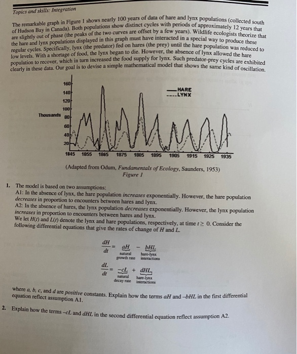
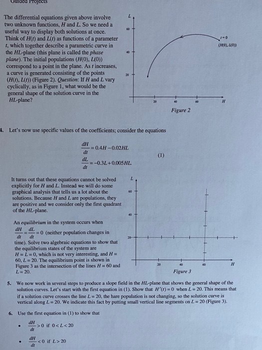
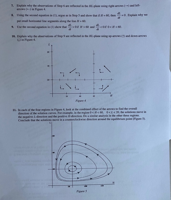
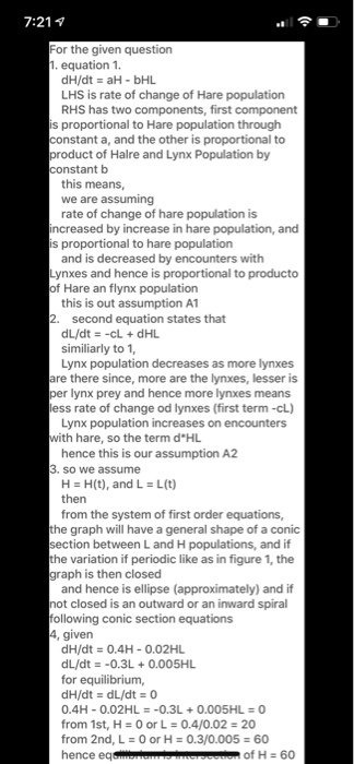
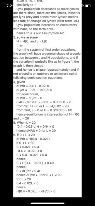
The remarkable graph in Figure I shows nearly 100 years of data of hare and lynx populations (collected south of Hudson Bay in Canada). Both populations show distinct cycles with periods of approximately 12 years that are slightly out of phase (the peaks of the two curves are offset by a few years). Wildlife ecologists theorize that clearly in these data. Our goal is to devise a simple mathematical model that shows the same kind of oscillation. Topics and skills: Integration the hare and lynx populations displayed in this graph must have interacted in a special way to produce thrice! low levels. With a shortage of food, the lynx began to die. However, the absence of lynx allowed the hare 160 HARE LYNX 1401 120 100 Thousands 80 60 W 405 . 20 1845 1855 1865 1875 1885 1895 1905 1915 1925 1935 (Adapted from Odum, Fundamentals of Ecology, Saunders, 1953) Figure / 1. The model is based on two assumptions: Al: In the absence of lynx, the hare population increases exponentially. However, the hare population decreases in proportion to encounters between hares and lynx. A2: In the absence of hares, the lynx population decreases exponentially. However, the lynx population increases in proportion to encounters between hares and lynx. We let H() and L(I) denote the lynx and hare populations, respectively, at time I 0. Consider the following differential equations that give the rates of change of H and L dH dt aH natural growth rate DHL hare-lys interactions dL dt CL + DHL natural hare-lynx decay rate interactions where a, b, c, and d are positive constants. Explain how the terms aH andbHL in the first differential equation reflect assumption Al. 2. Explain how the terms -cl and dHL in the second differential equation reflect assumption A2. Projects 60 (FO), O)) 0 The differential equations given above involve two unknown functions, H and L. So we need a useful way to display both solutions at once. Think of H(o) and Lit) as functions of a parameter 1, which together describe a parametric curve in the HL-plane (this plane is called the phase plane). The initial populations (HO), LO)) correspond to a point in the plane. Ast increases, a curve is generated consisting of the points (H(),LO) (Figure 2). Question: If H and L vary cyclically, as in Figure 1, what would be the general shape of the solution curve in the HL-plane? 20 Figure 2 4. Let's now use specific values of the coefficients, consider the equations dH = 0.4H-0.02HL dt dL = -0.3L+0.005 HL. dt (1) L 60 It turns out that these equations cannot be solved explicitly for H and L. Instead we will do some graphical analysis that tells us a lot about the solutions. Because H and L are populations, they are positive and we consider only the first quadrant of the HL-plane. An equilibrium in the system occurs when dHdL = 0 (neither population changes in dr dt time). Solve two algebraic equations to show that the equilibrium states of the system are H=L=0, which is not very interesting, and H= 60, L = 20. The equilibrium point is shown in Figure 3 as the intersection of the lines H=60 and L-20. 40 60 H Figure 3 5. We now work in several steps to produce a slope field in the HL-plane that shows the general shape of the solution curves. Let's start with the first equation in (1). Show that H')=0 when L = 20. This means that if a solution curve crosses the line L = 20, the hare population is not changing, so the solution curve is vertical along L=20. We indicate this fact by putting small vertical line segments on L = 20 (Figure 3). 6. Use the first equation in (1) to show that dH > 0 if 0 20 7. Explain why the observations of Step 6 are reflected in the HL-plane using right-arrows (-) and left- arrows (--)in Figure 4. dL 8. Using the second equation in (1), argue as in Step 5 and show that if H=60, then = 0. Explain why we dt put small horizontal line segments along the line H = 60. dL dL 9. Use the second equation in (1) show that -> Oif H > 60 and O for 0 20 0.4 -0.02L 0 if 0 20 7. Explain why the observations of Step 6 are reflected in the HL-plane using right-arrows (-) and left- arrows (--)in Figure 4. dL 8. Using the second equation in (1), argue as in Step 5 and show that if H=60, then = 0. Explain why we dt put small horizontal line segments along the line H = 60. dL dL 9. Use the second equation in (1) show that -> Oif H > 60 and O for 0 20 0.4 -0.02L