We now provide you with code for simulating the model above $($see below$).$ This consists of two functions, which you can inspect below. All can be seen in the live docs. Read them to help answer the remainder of question $5,$ which is situated below the code.

parameterise$\_$basic$\_$model

solve

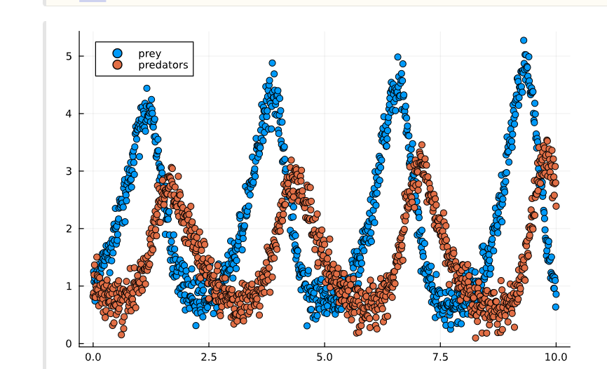
We also provide a variable data, that provides noisy data on the predator and prey populations taken by a biologist...

data$[$:$,1]$ contains the timepoints $($measured in years$)$ over which the data was taken

data$[$:$,2]$ represents the estimated prey population $($measured in hundreds, i$.$e$.$ data$[2,2]=3$ means $300$ estimated animals at timepoint $2)$ over these timepoints

data$[$:$,3]$ represents the predator population over these timepoints, measured in tens. $1001\backslash$times $3$ Matrix$\{$Float$64\}$:

$0\mathrm{.}00\mathrm{.}8253710\mathrm{.}820219$

$0\mathrm{.}011\mathrm{.}251260\mathrm{.}880475$

$0\mathrm{.}021\mathrm{.}074471\mathrm{.}19519$

$0\mathrm{.}031\mathrm{.}145951\mathrm{.}36702$

$0\mathrm{.}040\mathrm{.}740690\mathrm{.}820193$

$0\mathrm{.}050\mathrm{.}8032850\mathrm{.}802094$

$0\mathrm{.}061\mathrm{.}042340\mathrm{.}996427$

$$

$9\mathrm{.}950\mathrm{.}9602512\mathrm{.}89815$

$9\mathrm{.}960\mathrm{.}9586672\mathrm{.}57985$

$9\mathrm{.}971\mathrm{.}148992\mathrm{.}78071$

$9\mathrm{.}981\mathrm{.}096213\mathrm{.}08052$

$9\mathrm{.}990\mathrm{.}6355452\mathrm{.}79623$

$10\mathrm{.}00\mathrm{.}8571592\mathrm{.}38937.$ solve$($f::Function, tspan, x$0$::Vector$)$

Numerically solves the ODE x$($t$)=$ f$($x$($t$),$ t$)$

on the timespan whose start$/$end points are enclosed in tspan. Recall that x$$ denotes the time derivative of x$($t$),$ i$.$e$.$ dx$/$dt$.$

Example

solve$($f$,(0,10),[1,0])$

solves between t$=0$ and t$=10,$ using initial conditions x$0=[1,0].$ e$)$ How would the basic model change if we instead measured predators and prey in units of a single animal?

Hint: take $=\frac{Z}{100}$ and $=\frac{O}{10.}$

Can you rewrite the differential equation in terms of these two variables instead, using the chain rule?

f$)$ Build a function simulation$($p$).$ It must take in a vector of $4$ parameters $($e$.$g$.$ simulation$([1,2,3,4]).$ It must output a $1001\backslash$times $2$ matrix holding the solution of the differential equation: i$.$e$.$ the populations of prey $(1$st column$)$ and predators $(2$nd column$)$ over the timepoints range$(0,10,$step$=0\mathrm{.}01).$ The initial conditions can be $[1,1].$

g$)$ Build a function mse$($p$).$ It must take in a vector of $4$ parameters $($e$.$g$.$ mse$[1,2,3,4]).$ It must output the mean squared error between the model simulation, and the data provided in the variable data. The mean squared error is the sum of the squared residuals between the data and the simulation over all timepoints, divided by the number of timepoints.

h$)$ Use the gradient function provided below $($or not if you prefer!$)$ to implement a gradient descent algorithm, with stepsize $0\mathrm{.}01$

$.$ Run it$,$ starting from the initial parameter set p$0=[1,4,1,4].$ You have succeeded if you can use this algorithm to find a new parameter set pnew $=[$a$,$b$,$c$,$d$]$ that reduces the mean squared error by a factor of $3,$ as compared to p$0.$ Do two plots:

A comparison of the data and the simulation at p$0$

A comparison of the data and the simulation at pend.

Hint: to overlay two plots you can use the code:

p $=$ plot$()$

plot!$($p$,...)$

scatter!$($p$,...)$

where $...$ are the arguments you would usually provide to plot or scatter

If the algorithm doesn't effectively fit the data, why do you think this might be the case?

i$)$ Suppose you found parameter values that perfectly fitted the data $($mse $=0).$ Are these parameter values unique? i$.$e$.,$ could you find another set of parameter values that also perfectly fit the data?

gradient

gradient$($f::Function, x::Number$)$

Extracts the numerical gradient $(/$jacobian$/$multidimensional derivative$)$ of a function f$,$ evaluated at the vector x$.$ gradient uses the finite difference approximation

Conditions on f

f must accept a vector x of inputs, e$.$g$.$ f$([1,2,3].$ This vector is of length n$,$ where n is any number.

f must return a scalar output $($i$.$e$.$ a number, not a vector$)$