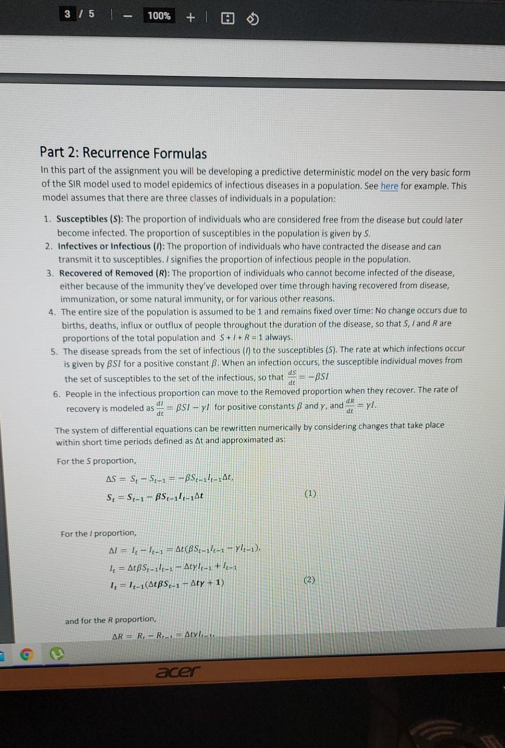
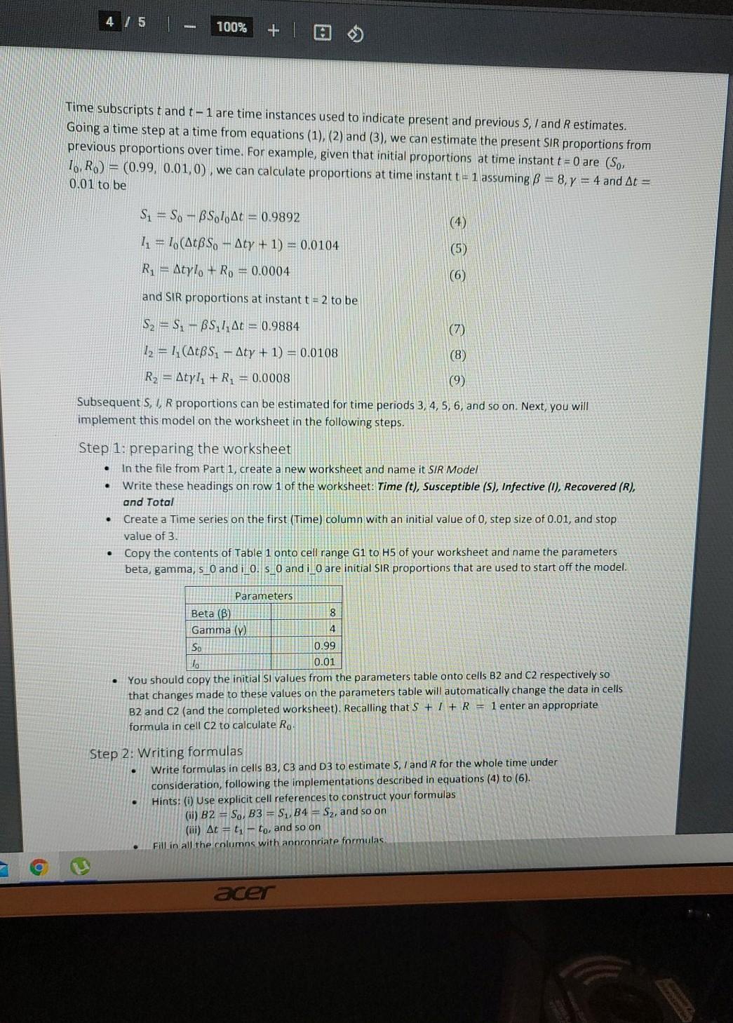
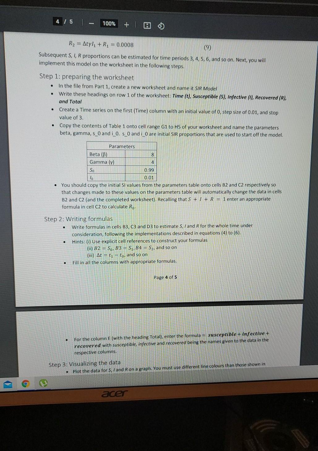
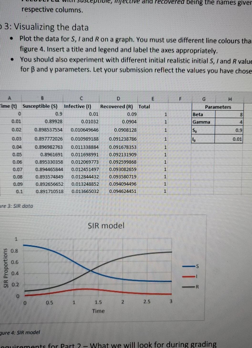
what formulas we need to use on cells b2 and c2 in step 1 and step 2

3 / 5 - 100% Part 2: Recurrence Formulas In this part of the assignment you will be developing a predictive deterministic model on the very basic form of the SIR model used to model epidemics of infectious diseases in a population. See here for example. This model assumes that there are three classes of individuals in a population: 1. Susceptibles (S): The proportion of individuals who are considered free from the disease but could later become infected. The proportion of susceptibles in the population is given by S. 2. Infectives or Infectious (1): The proportion of individuals who have contracted the disease and can transmit it to susceptibles. I signifies the proportion of infectious people in the population 3. Recovered of Removed (R): The proportion of individuals who cannot become infected of the disease, either because of the immunity they've developed over time through having recovered from disease, immunization, or some natural immunity, or for various other reasons. 4. The entire size of the population is assumed to be 1 and remains fixed over time: No change occurs due to births, deaths, influx or outflux of people throughout the duration of the disease, so that S, I and Rare proportions of the total population and S+ / + R = 1 always. 5. The disease spreads from the set of infectious (1) to the susceptibles (S). The rate at which infections occur is given by BSI for a positive constant . When an infection occurs, the susceptible individual moves from the set of susceptibles to the set of the infectious, so that -BST 6. People in the infectious proportion can move to the Removed proportion when they recover. The rate of di dR recovery is modeled as = BSI - yl for positive constants and y, and = yl. ds dt dt di The system of differential equations can be rewritten numerically by considering changes that take place within short time periods defined as At and approximated as: For the S proportion, AS = Si-S-1 = -S-11-1At, Se=S-1 - BS-11-140 (1) For the proportion, Al = 1,-1,-1 = At(BS-1/4-1 - 71.-1), 1 = AtBS-11-1 - Aty1-1 +14-1 1,=14-1(Atps-1 - Aty +1) (2) and for the R proportion, AR = R.-R.-1 = Atyl.-1. a acer 4 / 5 100% + Time subscriptstand t-1 are time instances used to indicate present and previous S, I and R estimates. Going a time step at a time from equations (1), (2) and (3), we can estimate the present SiR proportions from previous proportions over time. For example, given that initial proportions at time instant t = 0 are (So, To, R) = (0.99, 0.01,0), we can calculate proportions at time instant t = 1 assuming B = 8,7 = 4 and At = 0.01 to be (4) Si = So - BS.7 At = 0.9892 11 = 1. (Atso - Aty + 1) = 0.0104 R = Atylo + Rp = 0.0004 (5) (6) and SIR proportions at instant t = 2 to be S2 = $ - BS // At = 0.9884 (7) ) = 1, (S, - ty + 1) = 0.01 08 (8) R2 = Atyl +R; = 0.0008 (9) Subsequent S, I, R proportions can be estimated for time periods 3, 4, 5, 6, and so on. Next, you will implement this model on the worksheet in the following steps. Step 1: preparing the worksheet In the file from Part 1, create a new worksheet and name it SIR Model Write these headings on row 1 of the worksheet: Time (t), Susceptible (S), Infective (6), Recovered (R), and Total Create a Time series on the first (Time) column with an initial value of O, step size of 0.01, and stop value of 3. Copy the contents of Table 1 onto cell range G1 to H5 of your worksheet and name the parameters beta, gamma, s 0 and il 0. s_0 and i 0 are initial SiR proportions that are used to start off the model. . . Parameters Beta (B) 8 Gamma (v) 4 So 0.99 lo You should copy the initial si values from the parameters table onto cells B2 and C2 respectively so that changes made to these values on the parameters table will automatically change the data in cells B2 and C2 (and the completed worksheet). Recalling that S + I + R = 1 enter an appropriate formula in cell C2 to calculate Ro 0.01 . . Step 2: Writing formulas Write formulas in cells B3, C3 and D3 to estimate S, / and R for the whole time under consideration, following the implementations described in equations (4) to (6). Hints: (i) Use explicit cell references to construct your formulas (ii) B2 = So, B3 = $1,B4 = S2, and so on (iii) At = ti-to, and so on Fill in all the columns with annronriate formulas acer 4 / 5 100% + . R2 = Atyl: + R1 = 0.0008 (9) Subsequent S, I, R proportions can be estimated for time periods 3, 4, 5, 6, and so on. Next, you will implement this model on the worksheet in the following steps. Step 1: preparing the worksheet In the file from Part 1, create a new worksheet and name it SIR Model Write these headings on row 1 of the worksheet: Time (t), Susceptible (S), Infective (0), Recovered (R), and Total Create a Time series on the first (Time) column with an initial value of 0, step size of 0.01, and stop value of 3 Copy the contents of Table 1 onto cell range G1 to H5 of your worksheet and name the parameters beta, gamma, s_0 and i 0. s_0 and i 0 are initial SiR proportions that are used to start off the model. . Parameters Beta (B) 8 Gamma (v) 4 S. 0.99 lo 0.01 You should copy the initial Sl values from the parameters table onto cells B2 and C2 respectively so that changes made to these values on the parameters table will automatically change the data in cells B2 and C2 (and the completed worksheet). Recalling that S + I + R = 1 enter an appropriate formula in cell C2 to calculate Ro . . Step 2: Writing formulas Write formulas in cells B3, C3 and D3 to estimate S, I and R for the whole time under consideration, following the implementations described in equations (4) to (6). Hints: (0) Use explicit cell references to construct your formulas (ii) B2 = S., B3 = S1,B4 = S2, and so on (iii) At = ti to, and so on Fill in all the columns with appropriate formulas. . Page 4 of 5 . For the column E (with the heading Total), enter the formula = susceptible + infective + recovered with susceptible, infective and recovered being the names given to the data in the respective columns. Step 3: Visualizing the data Plot the data for S, 7 and Ron a graph. You must use different line colours than those shown in acer -POL mjecuve and recovered being the names giver respective columns. 3: Visualizing the data Plot the data for S, I and Ron a graph. You must use different line colours tha figure 4. Insert a title and legend and label the axes appropriately. You should also experiment with different initial realistic initial S, I and R value for B and y parameters. Let your submission reflect the values you have chose F G Parameters Beta 1 8 1 Gamma 1 S, 1 B C D E ime (0) Susceptible (s) Infective (0) Recovered (R) Total 0.9 0.01 0.09 0.89928 0.01032 0.0904 0.02 0.898537554 0.010649616 0.0908128 0.03 0.897772026 0.010989188 0.091238786 0.896982763 0.011338884 0.091678353 0.05 0.8961691 0.011698991 0.092131909 0.012069773 0.092599868 0.012451497 0.093082659 0.893574949 0.012844432 0.093580719 0.892656652 0,013248852 0.094094496 0.891710518 0.013665032 0.094624451 1 1 1 1 1 re 3: SIR doto SIR model SIR Proportions ili 0.2 R 0 0.5 1 2 3 Time gure 4. SIR model nauirements for Part 2 - What we will look for during grading 3 / 5 - 100% Part 2: Recurrence Formulas In this part of the assignment you will be developing a predictive deterministic model on the very basic form of the SIR model used to model epidemics of infectious diseases in a population. See here for example. This model assumes that there are three classes of individuals in a population: 1. Susceptibles (S): The proportion of individuals who are considered free from the disease but could later become infected. The proportion of susceptibles in the population is given by S. 2. Infectives or Infectious (1): The proportion of individuals who have contracted the disease and can transmit it to susceptibles. I signifies the proportion of infectious people in the population 3. Recovered of Removed (R): The proportion of individuals who cannot become infected of the disease, either because of the immunity they've developed over time through having recovered from disease, immunization, or some natural immunity, or for various other reasons. 4. The entire size of the population is assumed to be 1 and remains fixed over time: No change occurs due to births, deaths, influx or outflux of people throughout the duration of the disease, so that S, I and Rare proportions of the total population and S+ / + R = 1 always. 5. The disease spreads from the set of infectious (1) to the susceptibles (S). The rate at which infections occur is given by BSI for a positive constant . When an infection occurs, the susceptible individual moves from the set of susceptibles to the set of the infectious, so that -BST 6. People in the infectious proportion can move to the Removed proportion when they recover. The rate of di dR recovery is modeled as = BSI - yl for positive constants and y, and = yl. ds dt dt di The system of differential equations can be rewritten numerically by considering changes that take place within short time periods defined as At and approximated as: For the S proportion, AS = Si-S-1 = -S-11-1At, Se=S-1 - BS-11-140 (1) For the proportion, Al = 1,-1,-1 = At(BS-1/4-1 - 71.-1), 1 = AtBS-11-1 - Aty1-1 +14-1 1,=14-1(Atps-1 - Aty +1) (2) and for the R proportion, AR = R.-R.-1 = Atyl.-1. a acer 4 / 5 100% + Time subscriptstand t-1 are time instances used to indicate present and previous S, I and R estimates. Going a time step at a time from equations (1), (2) and (3), we can estimate the present SiR proportions from previous proportions over time. For example, given that initial proportions at time instant t = 0 are (So, To, R) = (0.99, 0.01,0), we can calculate proportions at time instant t = 1 assuming B = 8,7 = 4 and At = 0.01 to be (4) Si = So - BS.7 At = 0.9892 11 = 1. (Atso - Aty + 1) = 0.0104 R = Atylo + Rp = 0.0004 (5) (6) and SIR proportions at instant t = 2 to be S2 = $ - BS // At = 0.9884 (7) ) = 1, (S, - ty + 1) = 0.01 08 (8) R2 = Atyl +R; = 0.0008 (9) Subsequent S, I, R proportions can be estimated for time periods 3, 4, 5, 6, and so on. Next, you will implement this model on the worksheet in the following steps. Step 1: preparing the worksheet In the file from Part 1, create a new worksheet and name it SIR Model Write these headings on row 1 of the worksheet: Time (t), Susceptible (S), Infective (6), Recovered (R), and Total Create a Time series on the first (Time) column with an initial value of O, step size of 0.01, and stop value of 3. Copy the contents of Table 1 onto cell range G1 to H5 of your worksheet and name the parameters beta, gamma, s 0 and il 0. s_0 and i 0 are initial SiR proportions that are used to start off the model. . . Parameters Beta (B) 8 Gamma (v) 4 So 0.99 lo You should copy the initial si values from the parameters table onto cells B2 and C2 respectively so that changes made to these values on the parameters table will automatically change the data in cells B2 and C2 (and the completed worksheet). Recalling that S + I + R = 1 enter an appropriate formula in cell C2 to calculate Ro 0.01 . . Step 2: Writing formulas Write formulas in cells B3, C3 and D3 to estimate S, / and R for the whole time under consideration, following the implementations described in equations (4) to (6). Hints: (i) Use explicit cell references to construct your formulas (ii) B2 = So, B3 = $1,B4 = S2, and so on (iii) At = ti-to, and so on Fill in all the columns with annronriate formulas acer 4 / 5 100% + . R2 = Atyl: + R1 = 0.0008 (9) Subsequent S, I, R proportions can be estimated for time periods 3, 4, 5, 6, and so on. Next, you will implement this model on the worksheet in the following steps. Step 1: preparing the worksheet In the file from Part 1, create a new worksheet and name it SIR Model Write these headings on row 1 of the worksheet: Time (t), Susceptible (S), Infective (0), Recovered (R), and Total Create a Time series on the first (Time) column with an initial value of 0, step size of 0.01, and stop value of 3 Copy the contents of Table 1 onto cell range G1 to H5 of your worksheet and name the parameters beta, gamma, s_0 and i 0. s_0 and i 0 are initial SiR proportions that are used to start off the model. . Parameters Beta (B) 8 Gamma (v) 4 S. 0.99 lo 0.01 You should copy the initial Sl values from the parameters table onto cells B2 and C2 respectively so that changes made to these values on the parameters table will automatically change the data in cells B2 and C2 (and the completed worksheet). Recalling that S + I + R = 1 enter an appropriate formula in cell C2 to calculate Ro . . Step 2: Writing formulas Write formulas in cells B3, C3 and D3 to estimate S, I and R for the whole time under consideration, following the implementations described in equations (4) to (6). Hints: (0) Use explicit cell references to construct your formulas (ii) B2 = S., B3 = S1,B4 = S2, and so on (iii) At = ti to, and so on Fill in all the columns with appropriate formulas. . Page 4 of 5 . For the column E (with the heading Total), enter the formula = susceptible + infective + recovered with susceptible, infective and recovered being the names given to the data in the respective columns. Step 3: Visualizing the data Plot the data for S, 7 and Ron a graph. You must use different line colours than those shown in acer -POL mjecuve and recovered being the names giver respective columns. 3: Visualizing the data Plot the data for S, I and Ron a graph. You must use different line colours tha figure 4. Insert a title and legend and label the axes appropriately. You should also experiment with different initial realistic initial S, I and R value for B and y parameters. Let your submission reflect the values you have chose F G Parameters Beta 1 8 1 Gamma 1 S, 1 B C D E ime (0) Susceptible (s) Infective (0) Recovered (R) Total 0.9 0.01 0.09 0.89928 0.01032 0.0904 0.02 0.898537554 0.010649616 0.0908128 0.03 0.897772026 0.010989188 0.091238786 0.896982763 0.011338884 0.091678353 0.05 0.8961691 0.011698991 0.092131909 0.012069773 0.092599868 0.012451497 0.093082659 0.893574949 0.012844432 0.093580719 0.892656652 0,013248852 0.094094496 0.891710518 0.013665032 0.094624451 1 1 1 1 1 re 3: SIR doto SIR model SIR Proportions ili 0.2 R 0 0.5 1 2 3 Time gure 4. SIR model nauirements for Part 2 - What we will look for during grading