what is the differences between these two code ? both of them for plots Gradient Descent algorithm for two vectors and using the same functions

However the the Graphs are different !!!! are both of them correct ? if they are correct then why the graph is different?

Please give me simple answers and by details so I can understand : becuase i think im confused between vectors and the way of ploting

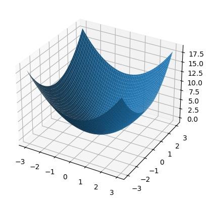
First code :-

import numpy as np from mpl_toolkits.mplot3d import Axes3D import matplotlib.pyplot as plt

class GradientDescent: def __init__(self, function, gradient, initial_solution, learning_rate=0.1, max_iter=100, tolerance=0.0000001): self.function = function self.gradient= gradient self.solution = initial_solution self.learning_rate = learning_rate self.max_iter = max_iter self.tolerance = tolerance def run(self): t = 0 while t

return self.solution, self.function(*self.solution)

def fun2(x, y): return x**2 + y**2

def gradient2(x, y): return np.array([2*x, 2*y])

bounds = [-3, 3]

fig = plt.figure() ax = fig.add_subplot(111, projection='3d')

X = np.linspace(bounds[0], bounds[1], 100) Y = np.linspace(bounds[0], bounds[1], 100) X, Y = np.meshgrid(X, Y) Z = fun2(X, Y) ax.plot_surface(X, Y, Z)

random_solution = np.random.uniform(bounds[0], bounds[1], size=2)

gd = GradientDescent(fun2, gradient2, random_solution)

best_solution, best_value = gd.run()

ax.scatter(best_solution[0], best_solution[1], best_value, color='r', s=100)

plt.show()

*****************************************************************************************************************************************

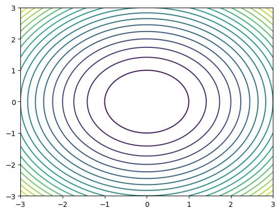
Second code :-

import numpy as np from matplotlib import pyplot as plt

class GradientDescent: def __init__(self, function, gradient, initial_solution, learning_rate=0.1, max_iter=100, tolerance=0.0000001): self.function = function self.gradient = gradient self.solution = initial_solution self.learning_rate = learning_rate self.max_iter = max_iter self.tolerance = tolerance def run(self): t = 0 while t

def fun1(x, y): return x ** 2 + y ** 2

def gradient1(x, y): return np.array([2 * x, 2 * y])

bounds = [-3, 3]

plt.figure()

x, y = np.meshgrid(np.linspace(bounds[0], bounds[1], 100), np.linspace(bounds[0], bounds[1], 100)) z = fun1(x, y) plt.contour(x, y, z,levels=20)

random_solution = np.random.uniform(bounds[0], bounds[1], size=2)

gd = GradientDescent(fun1, gradient1, random_solution)

best_solution, best_value = gd.run()

plt.plot(best_solution[0], best_solution[1])