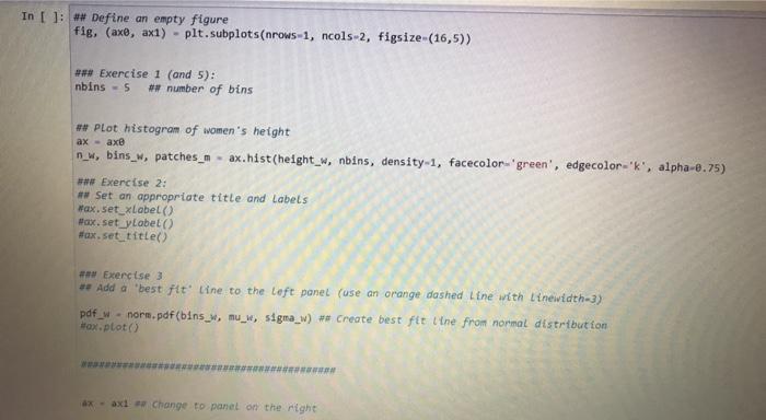
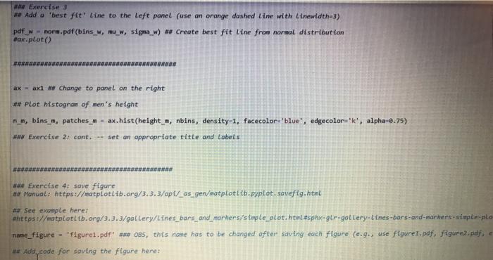
Workspace 2: Plot histograms 1: Set the number of bins (nbins) to 10 2. Set appropriate labels and titles (obs, do this for the panel on the right as well) 3: Add a best-fit line to the panel on the left (hint, use variables pdf_x and bins_x - note that is called something else in your code) 4. Save the figure (hint, change the name of the figure) 5. Test the meaning of nbins. Save a figure with nbins - 10 and nbins = 50 6. Change to a much larger dataset in workspace 1 and create a new set of figures using the code in workspace 2 (hint, try 1 million random numbers) In [ ]: ## Define an empty figure fig. (axe, axi) - plt.subplots(nrows-1, ncols-2, figsize-(16,5)) Exercise 1 (and 5): nbins - 5 ## number of bins ## Plot histogram of women's height ax - axe n_w, bins_w, patches_max.hist(height_w, nbins, density-1, facecolor-'green', edgecolor-'k', alpha-0.75) ### Exercise 2: ## Set an appropriate title and Labels Wax.set_xLabel() #ax.set_yLabel() #ax.set_title() * Exercise 3 * Add a 'best fit line to the left panel (use an orange dashed Line with linewidth-3) pdf_w - norm.pdf (bins_, mu_w, sigma_w) * Create best fit line from normal distribution ax.plot() axt Change to panel on the right # Exercise 3 ## Add o 'best fit line to the left panel (use an orange dashed Line with Linewidth-3) pdfw-norm.pdf(bins_w, mu_w, signa_w) we create best fit line from normal distribution #ax.plot() ax - axi ## Change to panel on the right ## Plot histogram of men's height num, bins_m, patches_max.hist(height_-, nbins, density-1, facecolor='blue', edgecolor 'k', alpha-0.75) ### Exercise 2: cont. set an appropriate title and Labels ### Exercise 4: save figure ** Manual: https://matplottib.org/3.3.3/apt/_as_gen/matplottib.pyplot. savefig.htel # See example here! https://matplotltb.org/3.3.3/gallery/Lines_bars_and_markers/simple plot.html#sphyglr-gallery-Lines-bars-and-market-simple-plo name_figure - 'figure1.pdf moss, this name has to be changed after saving each figure (e.g., use figure 1. pdf, figure2.pdf, * Add code for saving the figure here: Workspace 2: Plot histograms 1: Set the number of bins (nbins) to 10 2. Set appropriate labels and titles (obs, do this for the panel on the right as well) 3: Add a best-fit line to the panel on the left (hint, use variables pdf_x and bins_x - note that is called something else in your code) 4. Save the figure (hint, change the name of the figure) 5. Test the meaning of nbins. Save a figure with nbins - 10 and nbins = 50 6. Change to a much larger dataset in workspace 1 and create a new set of figures using the code in workspace 2 (hint, try 1 million random numbers) In [ ]: ## Define an empty figure fig. (axe, axi) - plt.subplots(nrows-1, ncols-2, figsize-(16,5)) Exercise 1 (and 5): nbins - 5 ## number of bins ## Plot histogram of women's height ax - axe n_w, bins_w, patches_max.hist(height_w, nbins, density-1, facecolor-'green', edgecolor-'k', alpha-0.75) ### Exercise 2: ## Set an appropriate title and Labels Wax.set_xLabel() #ax.set_yLabel() #ax.set_title() * Exercise 3 * Add a 'best fit line to the left panel (use an orange dashed Line with linewidth-3) pdf_w - norm.pdf (bins_, mu_w, sigma_w) * Create best fit line from normal distribution ax.plot() axt Change to panel on the right # Exercise 3 ## Add o 'best fit line to the left panel (use an orange dashed Line with Linewidth-3) pdfw-norm.pdf(bins_w, mu_w, signa_w) we create best fit line from normal distribution #ax.plot() ax - axi ## Change to panel on the right ## Plot histogram of men's height num, bins_m, patches_max.hist(height_-, nbins, density-1, facecolor='blue', edgecolor 'k', alpha-0.75) ### Exercise 2: cont. set an appropriate title and Labels ### Exercise 4: save figure ** Manual: https://matplottib.org/3.3.3/apt/_as_gen/matplottib.pyplot. savefig.htel # See example here! https://matplotltb.org/3.3.3/gallery/Lines_bars_and_markers/simple plot.html#sphyglr-gallery-Lines-bars-and-market-simple-plo name_figure - 'figure1.pdf moss, this name has to be changed after saving each figure (e.g., use figure 1. pdf, figure2.pdf, * Add code for saving the figure here


