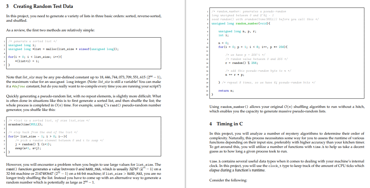
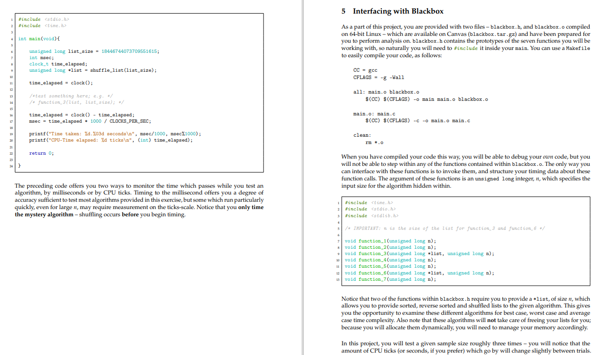
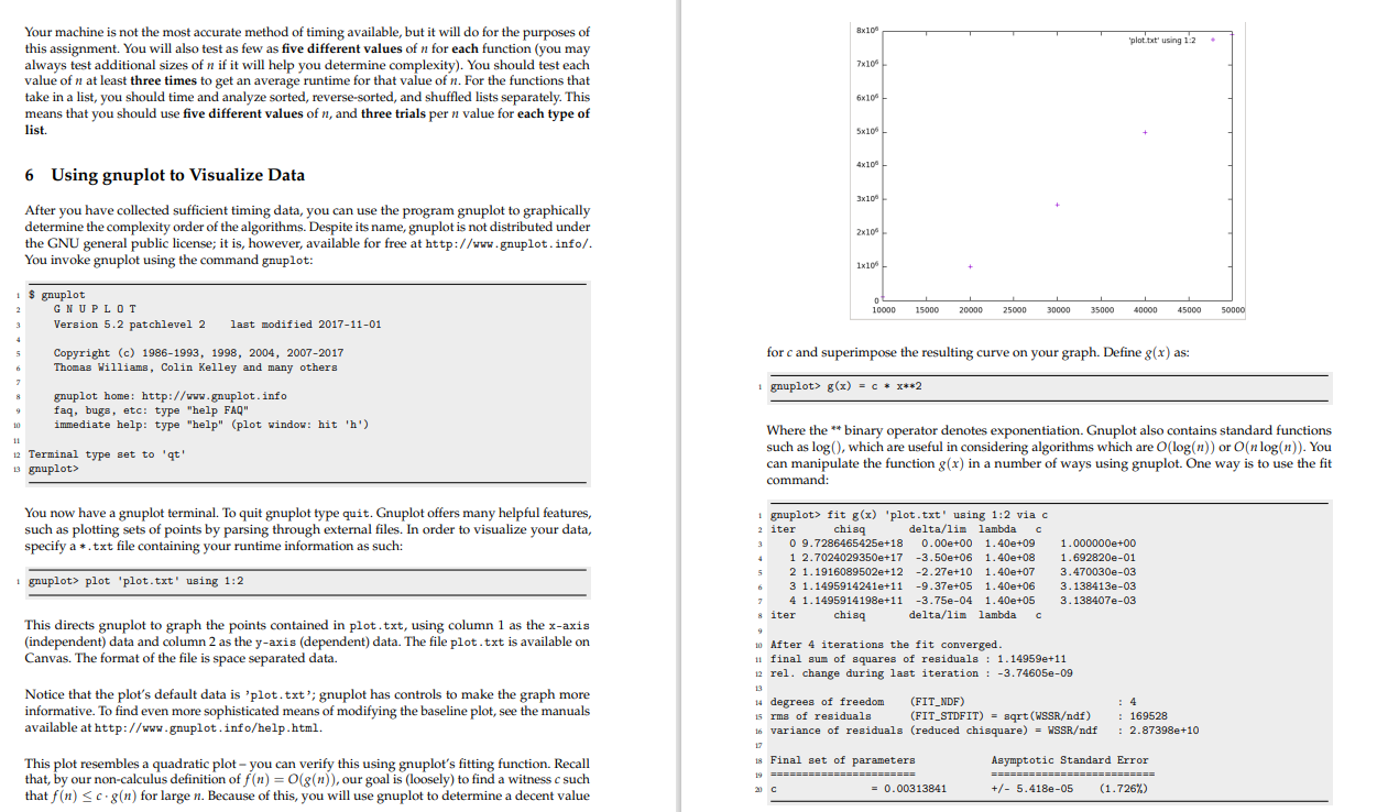
Write a program that interfaces with the blackbox: it should call the functions with different n-values and record the runtime of each call. I don't know where to start when writing a program to take different n-values of different functions.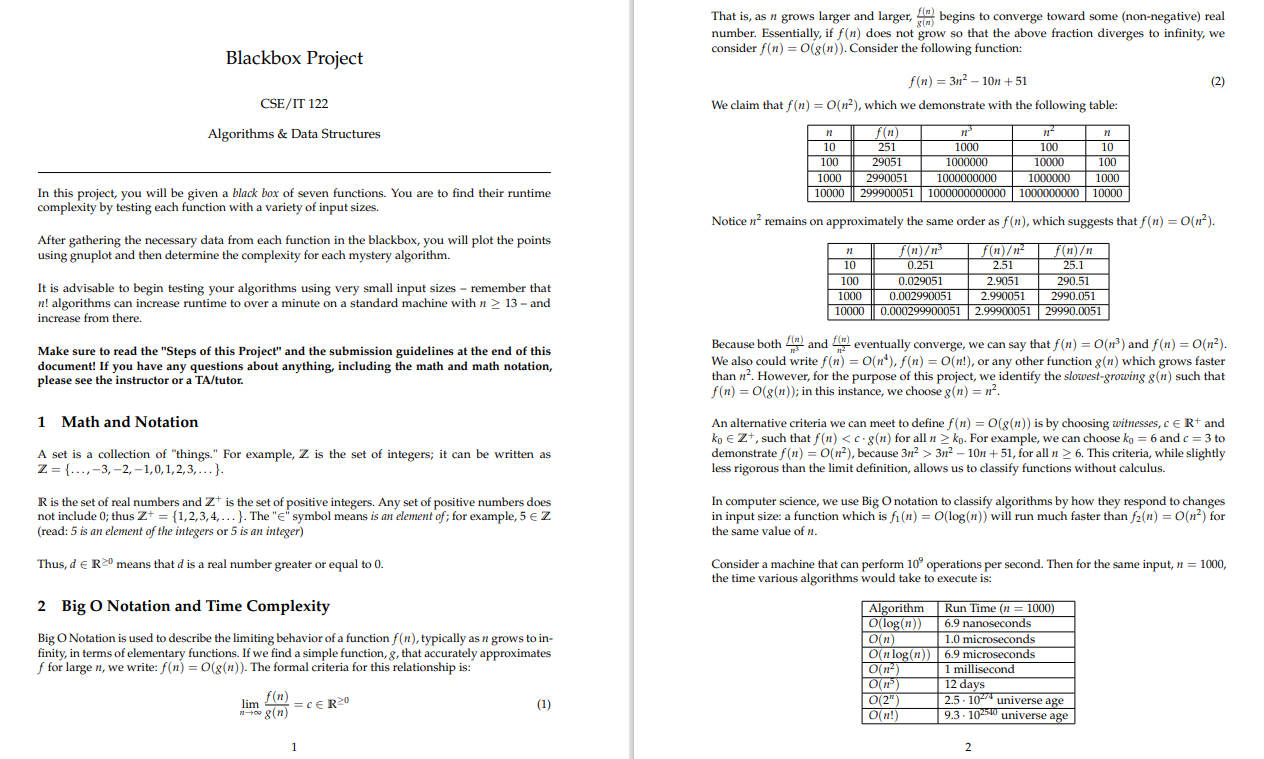

That is, as n grows larger and larger, flm begins to converge toward some (non-negative) real number. Essentially, if f(n) does not grow so that the above fraction diverges to infinity, we consider f(n) = 0(8(n)). Consider the following function: Blackbox Project (2) f(n) = 312 - 10n +51 We claim that f(n) = O(n), which we demonstrate with the following table: CSE/IT 122 Algorithms & Data Structures n 10 100 1000 10000 f(n) 251 1000 1000000 2990051 1000000000 299900051 1000000000000 29051 n- 100 10 10.0.0.0 100 1000000 1000 1000000000 10000 In this project, you will be given a black box of seven functions. You are to find their runtime complexity by testing each function with a variety of input sizes. Notice n remains on approximately the same order as f(n), which suggests that f(n) = O(n). After gathering the necessary data from each function in the blackbox, you will plot the points using gnuplot and then determine the complexity for each mystery algorithm. It is advisable to begin testing your algorithms using very small input sizes - remember that n! algorithms can increase runtime to over a minute on a standard machine with n > 13 - and increase from there. n f(n)/ f(n) 10 0.251 2.51 100 0.029051 2.9051 1000 0.002990051 2.990051 10000 0.000299900051 2.99900051 f(n) 25.1 290.51 2990.051 29990.0051 Make sure to read the "Steps of this project" and the submission guidelines at the end of this document! If you have any questions about anything, including the math and math notation, please see the instructor or a TA/tutor. Because both fm) and feventually converge, we can say that f(n) = O(n?) and f(n) = O(n). We also could write f(n) = O(n), f(n) = O(n!), or any other function g(n) which grows faster than n?. However, for the purpose of this project, we identify the slowest-growing 8(n) such that f(n) = 0(s(n)); in this instance, we choose g(n) = 12. 1 Math and Notation A set is a collection of "things." For example, Z is the set of integers; it can be written as Z = {..., -3, -2, -1,0,1,2,3,...}. An alternative criteria we can meet to define f(n) = 0(g(n)) is by choosing witnesses, ce R+ and ko Zt, such that f(n) 3n2 - 10n +51, for all n > 6. This criteria, while slightly less rigorous than the limit definition, allows us to classify functions without calculus. R is the set of real numbers and Zt is the set of positive integers. Any set of positive numbers does not include 0; thus Z+ = {1,2,3,4,... }. The "e" symbol means is an element of; for example, 5 Z (read: 5 is an element of the integers or 5 is an integer) In computer science, we use Big O notation to classify algorithms by how they respond to changes in input size: a function which is fi(n) = O(log(n)) will run much faster than f(n) = O(n) for the same value of n. Thus, de Romeans that d is a real number greater or equal to 0. Consider a machine that can perform 10 operations per second. Then for the same input, n = 1000, the time various algorithms would take to execute is: 2 Big O Notation and Time Complexity Big O Notation is used to describe the limiting behavior of a function f(n), typically as n grows to in- finity, in terms of elementary functions. If we find a simple function, g, that accurately approximates for large n, we write: f(n) = (g(n)). The formal criteria for this relationship is: Algorithm O(log(n)) On On log(n)) O(12) OP) O(2") On!) Run Time (n = 1000) 6.9 nanoseconds 1.0 microseconds 6.9 microseconds 1 millisecond 12 days 2.5. 10% universe age 9.3 - 102540 universe age f(n) lim 1 + g(n) =CERO (1) 1 3 Creating Random Test Data 1 2 In this project, you need to generate a variety of lists in three basic orders: sorted, reverse-sorted, and shuffled. /* random_number: generates a pseudo-random long unsigned between 0 and 2-64 - 1 3 seed random() with srandom(time(NULL)) before you call this */ 4 unsigned long random_number(void) { 5 As a review, the first two methods are relatively simple: 6 2 unsigned long n, p, r; int i; 8 9 /* generate a sorted list */ 2 unsigned long i; 3 unsigned long list = malloc(list_size + sizeof(unsigned long)); n = 0; for (i = 0; p = 1; i 0; i--){ /* pick a random element between 0 and i to swap / j = random() % (i+1); 8 swap(a+1, a+j); 9) In this project, you will analyze a number of mystery algorithms to determine their order of complexity. Naturally, this process necessitates some way for you to assess the runtime of various functions depending on their input size, preferably with higher accuracy than your kitchen timer. To get around this, you will utilize a number of functions with time.h to help us take a decent guess as to how long a given process took to run. 7 time. h contains several useful data types when it comes to dealing with your machine's internal clock. In this project, you will use the clock_t type to keep track of the amount of CPU ticks which elapse during a function's runtime. However, you will encounter a problem when you begin to use large values for list_size. The rand() function generates a value between 0 and RAND_MAX, which is usually 32767 (21 1) on a 32-bit machine or 2147483647 (231 - 1) on a 64-bit machine; if list_size > RAND_MAX, you are no longer truly shuffling the list. Instead you have to come up with an alternative way to generate a random number which is potentially as large as 264 - 1. Consider the following: 5 Interfacing with Blackbox #include #include 2 3 4 5 int main(void) { As a part of this project, you are provided with two files - blackbox.h, and blackbox.o compiled on 64-bit Linux - which are available on Canvas (blackbox.tar.gz) and have been prepared for you to perform analysis on blackbox.h contains the prototypes of the seven functions you will be working with, so naturally you will need to #include it inside your main. You can use a Makefile to easily compile your code, as follows: 6 unsigned long list_size = 18446744073709551615; int maec; clock_t time_elapsed; unsigned long list = shuffle_list (list_size); 8 9 CC = gcc 10 CFLAGS = -8 -Wall 11 time_elapsed - clock(); 12 13 /*test something here; e.g. */ /* function_3(list, list_size); */ all: main.o blackbox.o $(CC) $ (CFLAGS) - main main.o blackbox.o 14 15 16 time_elapsed = clock() - time_elapsed; msec = time_elapsed - 1000 / CLOCKS_PER_SEC; main.o: main.c $(CC) $ (CFLAGS) -C-o main.o main.c 17 18 printf("Time taken: %0.%03d seconds ", msec/1000, msec%1000); printf("CPU-Time elapsed: %d ticks ", (int) time_elapsed); 21 clean: rm .0 21 22 return 0; 23 24 } When you have compiled your code this way, you will be able to debug your own code, but you will not be able to step within any of the functions contained within blackbox.o. The only way you can interface with these functions is to invoke them, and structure your timing data about these function calls. The argument of these functions is an unsigned long integer, n, which specifies the input size for the algorithm hidden within. The preceding code offers you two ways to monitor the time which passes while you test an algorithm, by milliseconds or by CPU ticks. Timing to the millisecond offers you a degree of accuracy sufficient to test most algorithms provided in this exercise, but some which run particularly quickly, even for large n, may require measurement on the ticks-scale. Notice that you only time the mystery algorithm - shuffling occurs before you begin timing. #include #include #include 3 4 5 /* IMPORTANT: n is the size of the list for function_3 and function_6 */ ? void function_1(unsigned long n); & void function_2(unsigned long n); void function_3(unsigned long list, unsigned long n); 10 void function_4(unsigned long n); 11 void function_5(unsigned long n); 12 void function_6(unsigned long list, unsigned long n); 13 void function_7(unsigned long n); Notice that two of the functions within blackbox.h require you to provide a list of size n, which allows you to provide sorted, reverse sorted and shuffled lists to the given algorithm. This gives you the opportunity to examine these different algorithms for best case, worst case and average case time complexity. Also note that these algorithms will not take care of freeing your lists for you; because you will allocate them dynamically, you will need to manage your memory accordingly. In this project, you will test a given sample size roughly three times - you will notice that the amount of CPU ticks (or seconds, if you prefer) which go by will change slightly between trials. 8x100 plot.txt' using 12 7x106 Your machine is not the most accurate method of timing available, but it will do for the purposes of this assignment. You will also test as few as five different values of n for each function (you may always test additional sizes of n if it will help you determine complexity). You should test each value of n at least three times to get an average runtime for that value of n. For the functions that take in a list, you should time and analyze sorted, reverse-sorted, and shuffled lists separately. This means that you should use five different values of n, and three trials per n value for each type of list. . 6x106 5x100 4x100 3x10 6 Using gnuplot to Visualize Data After you have collected sufficient timing data, you can use the program gnuplot to graphically determine the complexity order of the algorithms. Despite its name, gnuplot is not distributed under the GNU general public license; it is, however, available for free at http://www.gnuplot.info/. You invoke gnuplot using the command gnuplot: 2x104 1x106 0 10000 15000 20000 25000 30000 35000 40000 45000 50000 1 $ gnuplot 2 GNUPLOT 3 Version 5.2 patchlevel 2 last modified 2017-11-01 Copyright (c) 1986-1993, 1998, 2004, 2007-2017 Thomas Williams, Colin Kelley and many others 5 for c and superimpose the resulting curve on your graph. Define g(x) as: 2 1 gnuplot> g(x) = C * x**2 8 gnuplot home: http://www.gnuplot.info 9 faq, bugs, etc: type "help FAQ" 10 immediate help: type "help" (plot window: hit 'h') 11 12 Terminal type set to 'qt' 13 gnuplot> Where the ** binary operator denotes exponentiation. Gnuplot also contains standard functions such as log(), which are useful in considering algorithms which are O(log(n)) or O(n log(n)). You can manipulate the function g(x) in a number of ways using gnuplot. One way is to use the fit command: You now have a gnuplot terminal. To quit gnuplot type quit. Gnuplot offers many helpful features, such as plotting sets of points by parsing through external files. In order to visualize your data, specify a *.txt file containing your runtime information as such: 1 gnuplot> plot 'plot.txt' using 1:2 ' 1 gnuplot> fit g(x) 'plot.txt' using 1:2 viac 2 iter chis delta/lim lambda 3 0 9.7286465425e+18 0.00e+00 1.40e+09 4 1 2.7024029350e+17 -3.50e+06 1.40e+08 + 5 2 1.1916089502e+12 -2.27e+10 1.40e+07 6 3 1.1495914241e+11 -9.37e+05 1.40e+06 4 1.1495914198e+11 -3.75e-04 1.40e+05 8 iter chisa delta/lim lambda 1.000000e+00 1.692820e-01 3.470030e-03 3.138413e-03 3.138407e-03 3 This directs gnuplot to graph the points contained in plot.txt, using column 1 as the x-axis (independent) data and column 2 as the y-axis (dependent) data. The file plot.txt is available on Canvas. The format of the file is space separated data. Notice that the plot's default data is 'plot.txt'; gnuplot has controls to make the graph more informative. To find even more sophisticated means of modifying the baseline plot, see the manuals available at http://www.gnuplot.info/help.html. 10 After 4 iterations the fit converged. 11 final sum of squares of residuals : 1.14959e+11 12 rel. change during last iteration : -3.74605-09 13 14 degrees of freedom (FIT_NDF) 15 rms of residuals (FIT_STDFIT) = sqrt(WSSRdf) 16 variance of residuals (reduced chisquare) = WSSRdf : 169528 : 2.87398e+10 This plot resembles a quadratic plot - you can verify this using gnuplot's fitting function. Recall that, by our non-calculus definition of f(n) =0(8(n)), our goal is (loosely) to find a witness c such that f(n) Sc.8(n) for large n. Because of this, you will use gnuplot to determine a decent value 18 Final set of parameters 19 ======================= 21 C = 0.00313841 Asymptotic Standard Error ================ ======== +/- 5.418e-05 (1.726%)