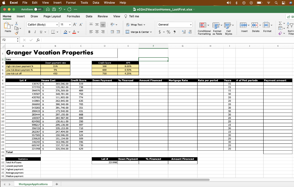
. Write an IF function in cell D9 that calculates the down payment for the mortgage. The down payment is 15% of the purchase price if the customer is considered high risk or 5% of the purchase price if considered low risk. The criteria to assess the risk of the loan is based on the credit score value in cell B6. Be sure to use the appropriate absolute or mixed cell references when referencing the input values in the range B4:B6. Then use the fill handle to copy the formula down, stopping in cell D28.

2. Enter a formula to calculate the percent financed in cell E9. The percent financed is the amount financed/purchase price. Next use the fill handle to copy the formula down, stopping in cell E28.

3. Enter a formula in cell F9 to calculate the amount financed. The amount financed is the purchase price minus the down payment. After entering the formula, use the fill handle to copy the formula down, stopping in cell F28.

4. Use the VLOOKUP function in cell G9, to look up the mortgage rate based on the customer credit score and the data in the range D4:E6. Be sure to use the appropriate absolute or mixed cell references. Use the fill handle to copy the formula down, stopping in cell G28.

5. Calculate the rate per period in cell H9. All mortgages being financed will be paid monthly. After completing the formula, use the fill handle to copy the formula down, stopping in cell H28.

6. Calculate the total number of payment periods in cell J10 based on the years financed in cell I9. After completing the formula, use the fill handle to copy the formula down, stopping in cell J28.

7. Use the PMT function to calculate the total monthly payment in cell K10 based on the periodic interest rate, number of periods, and amount financed. Ensure the results are a positive value, then use the fill handle to copy the function down, stopping in cell K28.

8. Use Quick Analysis to calculate the total of all payments in cell K29.

9. Use the appropriate statistical functions in the range B32:B36 to calculate descriptive statistics based on the row headings in the range A32:B36.

10. Use the XLOOKUP function in cell E32 to look up the employee number in cell D32 and return the corresponding down payment, % finances, and amount financed.

11. Use the appropriate function to insert the current date and time in cell B2.

Granger Vacation Properties Granger Vacation Properties