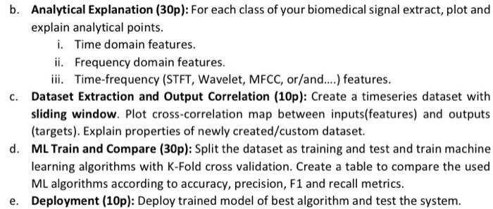
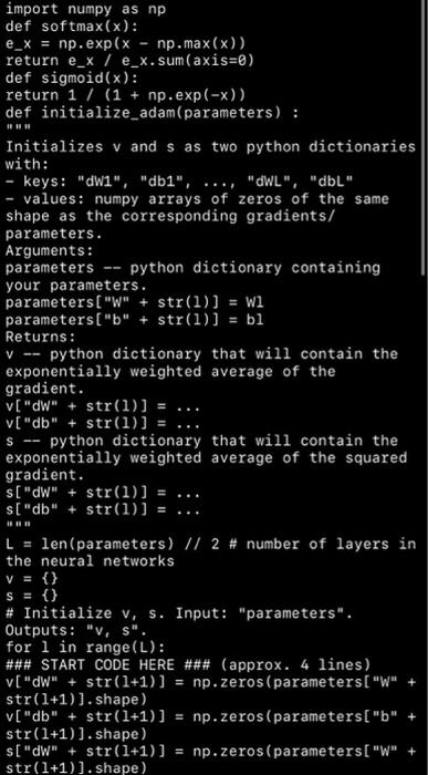
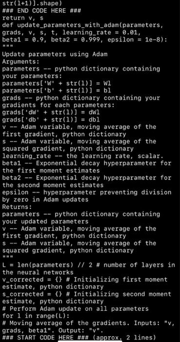
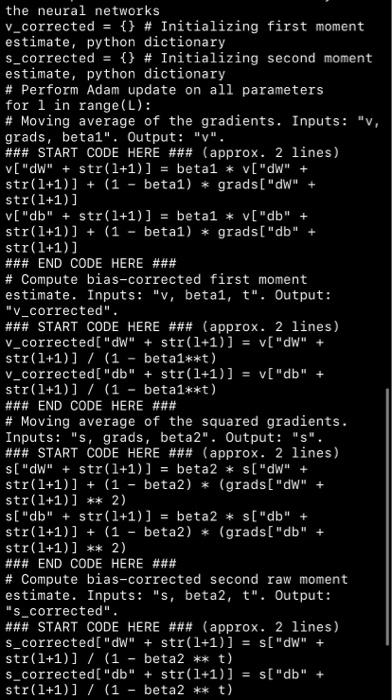
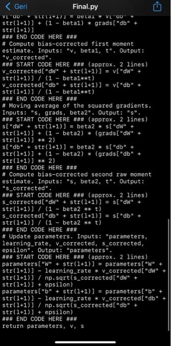
b. Analytical Explanation (30p): For each class of your biomedical signal extract, plot and explain analytical points. i. Time domain features. ii. Frequency domain features. iii. Time-frequency (STFT, Wavelet, MFCC, or/and....) features. C. Dataset Extraction and Output Correlation (10p): Create a timeseries dataset with sliding window. Plot cross-correlation map between inputs(features) and outputs (targets). Explain properties of newly created/custom dataset. d. ML Train and Compare (30p): Split the dataset as training and test and train machine learning algorithms with K-Fold cross validation. Create a table to compare the used ML algorithms according to accuracy, precision, F1 and recall metrics. e. Deployment (10p): Deploy trained model of best algorithm and test the system. V -- import numpy as np def softmax(x): e_X = np.exp(x - np.max(x)) return e_x / e_x. sum(axis=0) def sigmoid(x): return 1 / (1 + np.exp(-x)) def initialize_adam(parameters) : Initializes v and s as two python dictionaries with: - keys: "dW1", "db1", "dWL", "dbL" - values: numpy arrays of zeros of the same shape as the corresponding gradients/ parameters. Arguments: parameters python dictionary containing your parameters. parameters("W" + str(1) ) = Wl parameters("b" + str(1)) = bl Returns: python dictionary that will contain the exponentially weighted average of the gradient. v[ "dW" + str(1)) = v["db" + str(1)) = python dictionary that will contain the exponentially weighted average of the squared gradient. s["dW" + str(1)) s["db" + str(1)) = len (parameters) // 2 # number of layers in the neural networks v = {} S = {} # Initialize v, s. Input: "parameters". Outputs: "v, s". for i in range(L): ### START CODE HERE ### (approx. 4 lines) v["dW" + str(1+1)] = np.zeros(parameters[ "W" + str(1+1)). shape) v["db" + str(1+1)] = np.zeros(parameters["b" + str(1+1)].shape) S["dW" + str(1+1)] = np.zeros(parameters["W" + str(1+1)). shape) S- V - str(1+1)].shape) ### END CODE HERE ### return v, s def update_parameters_with_adam(parameters, grads, v, s, t, learning_rate = 0.01, beta1 = 0.9, beta2 = 0.999, epsilon = le-8): Update parameters using Adam Arguments: parameters python dictionary containing your parameters: parameters('W' + str(1)] = W1 parameters['b' + str(1)] = bl grads python dictionary containing your gradients for each parameters: grads['d' + str(1)] = dwl grads('db' + str(1)] = dbl Adam variable, moving average of the first gradient, python dictionary S -- Adam variable, moving average of the squared gradient, python dictionary learning_rate -- the learning rate, scalar. beta1 Exponential decay hyperparameter for the first moment estimates beta2 Exponential decay hyperparameter for the second moment estimates epsilon -- hyperparameter preventing division by zero in Adam updates Returns: parameters python dictionary containing your updated parameters V =- Adam variable, moving average of the first gradient, python dictionary Adam variable, moving average of the squared gradient, python dictionary L = len (parameters) // 2 # number of layers in the neural networks v_corrected = {} # Initializing first moment estimate, python dictionary s_corrected = {} # Initializing second moment estimate, python dictionary # Perform Adam update on all parameters for 1 in range(L): # Moving average of the gradients. Inputs: "v, grads, betal". Output: "V". ### START CODE HERE ### (approx. 2 lines) S =- the neural networks v_corrected = {} # Initializing first moment estimate, python dictionary s_corrected = {} # Initializing second moment estimate, python dictionary # Perform Adam update on all parameters for 1 in range(L): # Moving average of the gradients. Inputs: "v, grads, betal". Output: "v". ### START CODE HERE ### (approx. 2 lines) v["dW" + str(1+1)] beta1 * V["dW" + str(1+1)] + (1 - betal) * grads["dW" str(1+1)] V["db" + str(1+1)] = beta1 * v["db" str(1+1)] + (1 - betal) * grads["db" str(1+1)] ### END CODE HERE ### # Compute bias-corrected first moment estimate. Inputs: "v, betai, t". Output: "V_corrected". ### START CODE HERE ### (approx. 2 lines) v_corrected["dW" + str(1+1)] v["dW" + str(1+1)] / (1 - beta1**t) v_corrected["db" + str(1+1)] = v["db" str(1+1)] / (1 - beta1**t) ### END CODE HERE ### # Moving average of the squared gradients. Inputs: "s, grads, beta2". Output: "s". ### START CODE HERE ### (approx. 2 lines) s["dW" + str(1+1)] = beta2 * s["dW" + str(1+1)] + (1 - beta2) * (grads["dW" + str(1+1)] ** 2) s["db" + str(1+1)] = beta2 * s["db" + str(1+1)] + (1 - beta2) * (grads["db" str(1+1)] ** 2) ### END CODE HERE ### # Compute bias-corrected second raw moment estimate. Inputs: "s, beta2, t". Output: "s_corrected". ### START CODE HERE ### (approx. 2 lines) s_corrected["dW" + str(1+1)] = s["dW" + str(1+1)] / (1 beta2 ** t) $_corrected["db" + str(1+1)] s["db" str(1+1)] / (1 beta2 ** t) =
