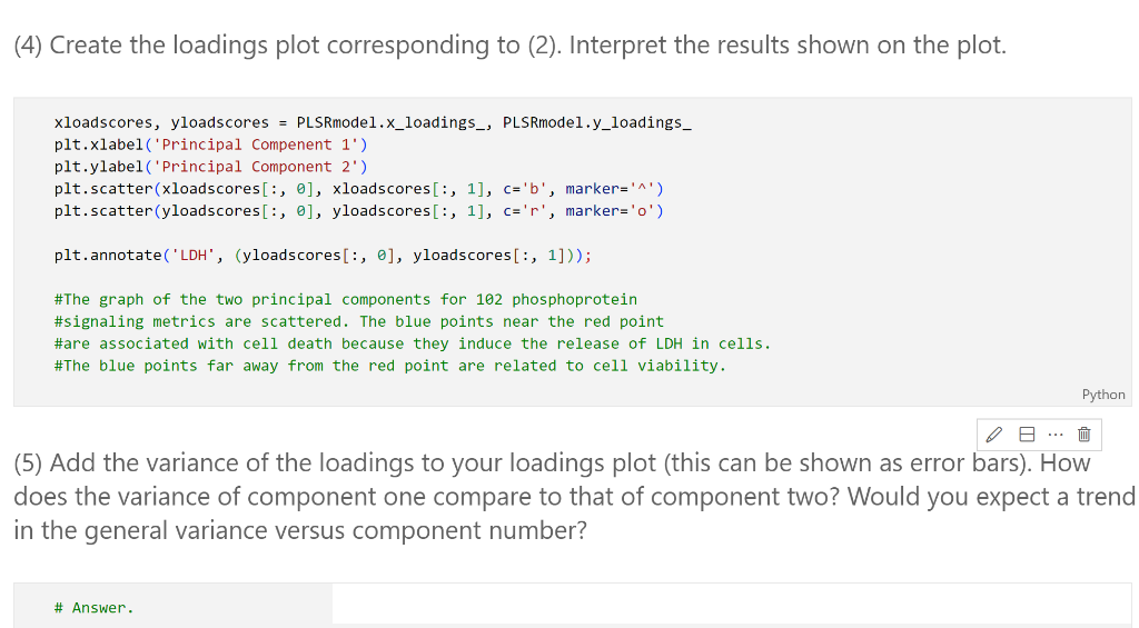
xloadscores, yloadscores = PLSRmodel.x_loadings_, PLSRmodel.y_loadings_ plt.xlabel('Principal compenent 1) plt.ylabel('Principal component 2 ') plt.scatter (xloadscores [:,0],x loadscores [:,1],c=bb, marker='^') plt.scatter(yloadscores [:,0], yloadscores [:,1],c=r, marker='o') plt.annotate('LDH', (yloadscores [:,0], yloadscores [:,1])); \#The graph of the two principal components for 102 phosphoprotein \#signaling metrics are scattered. The blue points near the red point \#are associated with cell death because they induce the release of LDH in cells. \#The blue points far away from the red point are related to cell viability. (5) Add the variance of the loadings to your loadings plot (this can be shown as error bars). How does the variance of component one compare to that of component two? Would you expect a trend in the general variance versus component number