Year Quarter Location CarClass Revenue NumCars

2018 Q1 Airport Economy 1011191 5650

2018 Q1 Downtown Economy 943509 5965

2017 Q4 Airport Economy 926382 5122

2016 Q3 Downtown Economy 777155 5280

2017 Q1 Downtown Economy 725178 4802

2017 Q4 Downtown Economy 710955 4529

2016 Q3 Airport Economy 708349 4649

2018 Q2 Airport Premium 697496 3726

2018 Q2 Airport SUV 697326 3918

2018 Q2 Airport Hybrid 697206 3781

2017 Q3 Downtown Economy 687341 4451

2018 Q1 Airport SUV 685728 3923

2018 Q1 Airport Premium 685524 3722

2018 Q1 Airport Hybrid 685013 3812

2017 Q3 Airport Hybrid 664684 3850

2017 Q3 Airport Premium 664353 3807

2017 Q3 Airport SUV 664219 4017

2017 Q2 Downtown Economy 646991 4218

2016 Q4 Airport Premium 640671 3816

2016 Q4 Airport Hybrid 640254 3898

2016 Q4 Airport SUV 623463 4034

2016 Q4 Airport Economy 618064 4031

2017 Q2 Airport Premium 605136 3486

2017 Q2 Airport SUV 604825 3709

2017 Q2 Airport Hybrid 604445 3578

2016 Q4 Downtown Premium 602216 3780

2016 Q4 Downtown Hybrid 601894 3869

2016 Q4 Downtown SUV 601517 4018

2018 Q2 Airport Economy 600780 3114

2017 Q3 Airport Economy 599375 3485

2018 Q2 Downtown Economy 580217 3532

2017 Q1 Airport Premium 571105 3351

2017 Q1 Airport SUV 570887 3552

2017 Q1 Airport Hybrid 570859 3446

2017 Q4 Airport Hybrid 546026 3054

2017 Q4 Airport SUV 545509 3168

2017 Q4 Airport Premium 545319 3022

2016 Q3 Downtown SUV 521701 3532

2016 Q3 Downtown Hybrid 521472 3376

2016 Q3 Downtown Premium 521308 3315

2016 Q4 Downtown Economy 513442 3389

2017 Q2 Downtown Hybrid 505147 3110

2017 Q2 Downtown SUV 505039 3187

2017 Q2 Downtown Premium 504891 3040

2017 Q1 Airport Economy 503650 3231

2017 Q3 Downtown SUV 499871 3134

2017 Q3 Downtown Hybrid 499161 3005

2017 Q3 Downtown Premium 499079 2947

2016 Q3 Airport Hybrid 488077 3029

2016 Q3 Airport Premium 487711 2945

2016 Q3 Airport SUV 487214 3138

2016 Q2 Airport Economy 484954 3272

2016 Q2 Downtown Hybrid 470951 3072

2016 Q2 Downtown SUV 470764 3213

2016 Q2 Downtown Premium 470558 3034

2016 Q1 Airport Economy 453665 3196

2018 Q1 Downtown Premium 436719 2500

2018 Q1 Downtown Hybrid 436650 2515

2018 Q1 Downtown SUV 436119 2643

2017 Q4 Downtown Premium 435682 2512

2017 Q4 Downtown Hybrid 435056 2569

2017 Q4 Downtown SUV 434943 2655

2017 Q1 Downtown Hybrid 428988 2675

2017 Q1 Downtown Premium 428691 2609

2017 Q1 Downtown SUV 428575 2744

2016 Q2 Downtown Economy 382948 2688

2017 Q2 Airport Economy 371631 2111

2016 Q1 Airport SUV 363309 2439

2016 Q1 Airport Hybrid 363062 2354

2016 Q1 Airport Premium 362646 2289

2016 Q1 Downtown Economy 361977 2658

2016 Q1 Downtown SUV 358062 2463

2016 Q1 Downtown Hybrid 357967 2373

2016 Q1 Downtown Premium 357693 2336

2018 Q2 Downtown Premium 332931 1837

2018 Q2 Downtown SUV 332851 1917

2018 Q2 Downtown Hybrid 332307 1873

2016 Q2 Airport Hybrid 306364 1943

2016 Q2 Airport Premium 305996 1895

2016 Q2 Airport SUV 305953 1987

This is the data and the instructions, i can't upload it as a document that's why i copied and pasted the data. pls share a link (google drive etc) so i can download the solution.

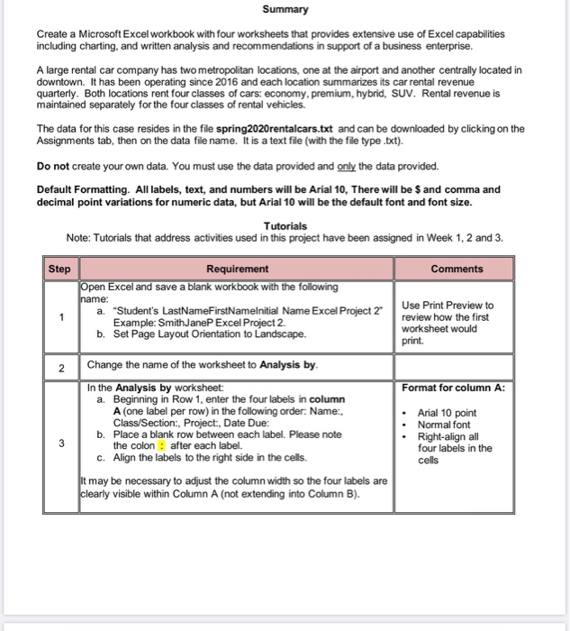
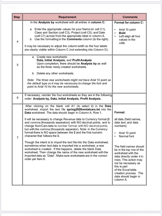
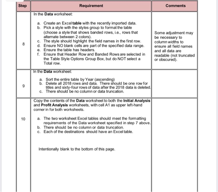
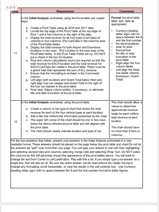
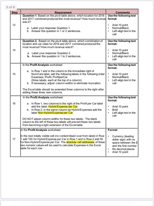
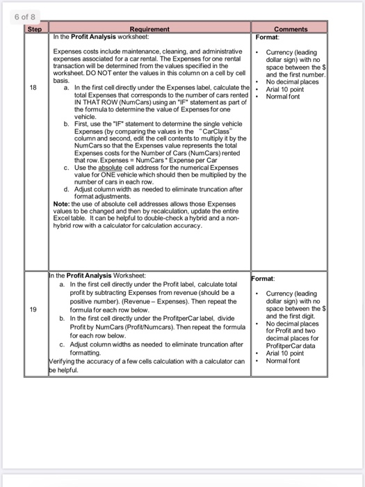
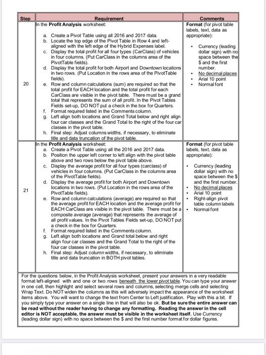
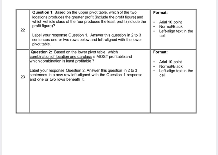
Summary Create a Microsoft Excel Workbook with four worksheets that provides extensive use of Excel capabilities including charting, and written analysis and recommendations in support of a business enterprise. A large rental car company has two metropolitan locations, one at the airport and another centrally located in downtown. It has been operating since 2016 and each location summarizes its car rental revenue quarterly. Both locations rent four classes of cars: economy, premium, hybrid, SUV. Rental revenue is maintained separately for the four classes of rental vehicles. The data for this case resides in the file spring 2020rentalcars.txt and can be downloaded by clicking on the Assignments tab, then on the data file name. It is a text file (with the file type.txt). Do not create your own data. You must use the data provided and only the data provided. Default Formatting. All labels, text, and numbers will be Arial 10. There will be $ and comma and decimal point variations for numeric data, but Arial 10 will be the default font and font size. Tutorials Note: Tutorials that address activities used in this project have been assigned in Week 1, 2 and 3. Step Comments Requirement Open Excel and save a blank workbook with the following name: a. "Student's LastNameFirstNamelnitial Name Excel Project 2 Example: Smith JaneP Excel Project 2 b. Set Page Layout Orientation to Landscape. Use Print Preview to review how the first worksheet would print. 2 Change the name of the worksheet to Analysis by. Format for column A: In the Analysis by worksheet: a. Beginning in Row 1, enter the four labels in column A (one label per row) in the following order: Name: Class/Section, Project:, Date Due: b. Place a blank row between each label. Please note the colon: after each label. c. Align the labels to the right side in the cells. Arial 10 point Normal font Right-align all four labels in the cells it may be necessary to adjust the column width so the four labels are clearly visible within Column A (not extending into Column B). Step Requirement In the Analysis by worksheet with all entries in column C: Comments Format for column C: Arial 10 point a. Enter the appropriate values for your Name (in cell C1). Class and Section (cell C3), Project (cell C5), and Date (cel C7) across from the appropriate label in column A. b. Use the formatting in the Comments column to the right) Bold Left-align all four values in the cells It may be necessary to adjust the column width so the four Labels are clearly visible within Column C (not extending into Column D). a Create new worksheets Data, Initial Analysis, and Profit Analysis Upon completion, there should be Analysis by as well as the three newly created worksheets b. Delete any other worksheets. Note: The three new worksheets might not have Arial 10 point as the default type so it may be necessary to change the font and point to Arial 10 for the new worksheets. If necessary, reorder the four worksheets so they are in the following order: Analysis by, Data, Initial Analysis, Profit Analysis. After clicking on the blank cell A1 (to select it) in the Data worksheet, import the text file spring 2020rentalcars.txt into the Data worksheet. The data should begin in Column A. Row 1. Format: all data (field names, data text, and data numbers) It will be necessary to change Revenue data to Currency format ($ and comma (thousands separators) with NO decimal points, and to change NumCars data to number format, with NO decimal points, but with the comma (thousands separator). Note: in the Currency format there is NO space between the S and the first numeric character that follows the $ Arial 10 point Normal font Though the intent is to import the text file into the Data worksheet sometimes when text data is imported into a worksheet, a new worksheet is created. If this happens, delete the blank Data worksheet. Then change the name of the new worksheet with the imported data as "Data". Make sure worksheets are in the correct order per Item 6. The field names should be in the top row of the worksheet with the data directly under it in rows. This action may not be necessary as this is part of the Excel table creation process. The data should begin in column A Step Requirement Comments In the Data worksheet: a. Create an Excel table with the recently imported data. b. Pick a style with the styles group to format the table (choose a style that shows banded rows, i.e., rows that alternate between 2 colors). The style should highlight the field names in the first row. d. Ensure NO blank cells are part of the specified data range. e. Ensure the table has headers. f. Ensure that Header Row and Banded Rows are selected in the Table Style Options Group Box, but do NOT select a Total row. Some adjustment may be necessary to column widths to ensure all field names and all data are readable (not truncated or obscured). In the Data worksheet: a. Sort the entire table by Year (ascending) b. Delete all 2018 rows and data. There should be one row for titles and sixty-four rows of data after the 2018 data is deleted. C. There should be no column or data truncation. Copy the contents of the Data worksheet to both the Initial Analysis and Profit Analysis worksheets, with cell A1 as upper left-hand corner in for both worksheets. a. The two worksheet Excel tables should meet the formatting requirements of the Data worksheet specified in step 7 above, b. There should be no column or data truncation. c. Each of the destinations should have an Excel table. Intentionally blank to the bottom of this page. 4 of 8 Step Requirement Comments In the Initial Analysis worksheet, using the Excel table just copied here: a. Create a Pivot Table using all 2016 and 2017 data. b. Locate the top edge of the Pivot Table at the top edge of Row 1 and a few columns to the right of the data. c. Display the total revenue for all four types (CarClass) of vehicles in four columns. (Put CarClass in the columns area of the Pivot Table fields) d. Display the total revenue for both Airport and Downtown locations in two rows. (Put Location in the rows area of the Pivot Table fields). In the Pivot Table Fields set-up. DO NOT put a check in the box for Quarter. e. Row and column calculations (sum) are required so that the total revenue for EACH location and the total revenue for EACH CarClass are visible in the pivot table. There must be a grand total that represents the sum of ALL revenue. 1. Ensure that the formatting is as listed in the Comments column 9. Left align both locations and Grand Total below them and right align four car classes and Grand Total to the right of the four car classes in the pivot table. h. Final step: Adjust column widths, if necessary, to eliminate title and data truncation of the pivot table. Format (for pivot table label, text, data as appropriate) Currency (leading dollar sign) with no space between the s and the first number No decimal places Arial 10 point Normal font No title or data truncation in the pivot table Right-align the five column labels. Left-align the three row labels Airport Downtown, Grand Total) In the Initial Analysis worksheet, using the pivot table: a. Create a column or bar type of chart that shows the total revenue for each of the four vehicle types at each location. b. Add a title that reflects the information presented by the chart. C. The upper left corner of the chart should be one or two rows below the above referenced pivot table and left-aligned with the pivot table d. The chart should clearly indicate location and type of car. The chart should allow a viewer to determine approximate revenue totals for each vehicle total revenue at each location. 112 The chart should have no more than 8 bars or columns For the two questions that follow, present your answers in the Initial Analysis worksheet in a very readable format. These answers should be placed on the page below the pivot table and chart Do not let the answers be "split over more than one page. You can type your answer in one cell, then highlighting and selecting several rows and columns, selecting merge cells and selecting Wrap Text. Do NOT widen the columns as this will adversely impact the appearance of the pivot tables above. You will want to change the text from Center to Left justification. Play with this a bit. If you simply type your answer on a single line, that will also be ok. Be sure the entire answer can be read without the reader having to change any formatting, scroll horizontally, or view the results in the cell contents box. Use Currency leading dollar sign) with no space between the $ and the first number format for dollar figures 5 of 8 Step Requirement Comments Question 1: Based on the pivot table above, which location for 2016 Use the following text and 2017 combined produced the most revenue? How much revenue format: was? Arial 10 point a. Label your response Question 1. Normal Black b. Answer this question in 1 or 2 sentences Left-align text in the cel Question 2. Based on the pivot table above, which combination of location and car class for 2016 and 2017 combined produced the most revenue? How much revenue was it? Use the following text format: a. Label your response Question 2 b. Answer this question in 1 to 2 sentences Arial 10 point Normal Black Left-align text in the cel In the Profit Analysis worksheet: Use the following text format: a. In Row 1 and in the column to the immediate right of NumCars label, add the following labels in the following order Expenses, Profit, ProfitperCar (three labels, each at the top of a column) b. If necessary, adjust column widths to eliminate truncation. . Arial 10 point Normal Black Left-align text in the cell The Excel table should be extended three columns to the right after adding these three new columns Use the following text format: 16 In the Profit Analysis worksheet: a. In Row 1, two columns to the right of the Profit per Car label add the label: Hybrid Expense per Car b. In Row 2, in the same column as Hybrid Expenses add the label Non-Hybrid Expense per Car. Arial 10 point Bold Left-align text in the cel Format: DO NOT adjust column widths for these two labels. The blank column to the left of these two labels will prevent these two labels from becoming a right extension of the Excel table. In the Profit Analysis worksheet: In the next totally visible cell (no content bleed over from label) in Row 11 add 100 for Hybrid Expense per Car in Row 1 and in Row 2 add 50 for Non-Hybrid Expense per Car. The absolute cell addresses of these two numeric values will be used to calculate Expenses in the Excel table for each row. Currency (leading dollar sign) with no space between the $ and the first number No decimal places Arial 10 point 6 of 8 Step Requirement In the Profit Analysis worksheet: Comments Format Expenses costs include maintenance, cleaning, and administrative Currency (leading expenses associated for a car rental. The Expenses for one rental dollar sign) with no transaction will be determined from the values specified in the space between the $ worksheet. DO NOT enter the values in this column on a cel by cel and the first number basis. No decimal places a In the first cell directly under the Expenses label, calculate thel. Arial 10 point total Expenses that corresponds to the number of cars rented . Normal font IN THAT ROW (NumCars) using an 'F statement as part of the formula to determine the value of Expenses for one vehicle. First, use the "IF statement to determine the single vehicle Expenses (by comparing the values in the "CarClass column and second edit the cell contents to multiply it by the NumCars so that the Expenses value represents the total Expenses costs for the Number of Cars (NumCars) rented that row. Expenses NumCars Expense per Car c. Use the absolute cel address for the numerical Expenses value for ONE vehicle which should then be multiplied by the number of cars in each row. d. Adjust column width as needed to eliminate truncation after format adjustments. Note: the use of absolute cell addresses allows those Expenses values to be changed and then by recalculation update the entire Excel table. It can be helpful to double-check a hybrid and a non- hybrid row with a calculator for calculation accuracy. Format: In the Profit Analysis Worksheet: a. In the first cell directly under the Profit label, calculate total profit by subtracting Expenses from revenue (should be a positive number). (Revenue - Expenses). Then repeat the formula for each row below. b. In the first cell directly under the ProfitperCar label, divide Profit by NumCars (Profit/Numcars). Then repeat the formula for each row below c. Adjust column widths as needed to eliminate truncation after formatting Verifying the accuracy of a few cells calculation with a calculator can e helpful Currency (leading dollar sign) with no space between the S and the first digit. No decimal places for Profit and two decimal places for ProfitperCar data Arial 10 point Normal font Step Requirement In the Profit Analysis worksheet: Comments Format (for pivot table labels, text, data as appropriate) Currency (leading dollar sign) with no space between the S and the first number No decimal places Arial 10 point Normal font 20 a. Create a Pivot Table using all 2016 and 2017 data. b. Locate the top edge of the Pivot Table in Row 4 and left- aligned with the left edge of the Hybrid Expenses label. c. Display the total profit for all four types (CarClass) of vehicles in four columns (Put CarClass in the columns area of the PivotTable fields). d Display the total profit for both Airport and Downtown locations in two rows. (Put Location in the rows area of the Pivot Table fields). e. Row and column calculations (sum) are required so that the total profit for EACH location and the total profit for each CarClass are visible in the pivot table. There must be a grand total that represents the sum of all profit. In the Pivot Tables Fields set-up. DO NOT put a check in the box for Quarters 1. Format required listed in the Comments column. 9. Left align both locations and Grand Total below and right align four car classes and the Grand Total to the right of the four car classes in the pivot table. h. Final step: Adjust columns widths, if necessary, to eliminate title and data truncation of the pivot table In the Profit Analysis worksheet: a. Create a Pivot Table using all the 2016 and 2017 data. b. Position the upper left corner to left align with the pivot table above and two rows below the pivot table above. c. Display the average profit for all four types (carclass) of vehicles in four columns (Put CarClass in the columns area of the Pivot Table fields). d. Display the average profit for both Airport and Downtown locations in two rows. (Put Location in the rows area of the Pivot Table fields) e. Row and column calculations (average) are required so that the average profit for EACH location and the average profit for EACH CarClass are visible in the pivot table. There must be a composite average (average) that represents the average of all profit values. In the Pivot Tables Fields set-up. DO NOT put a check in the box for Quarters 1. Format required listed in the Comments column 9. Left align both locations and Grand total below and right align four car classes and the Grand Total to the right of the four car classes in the pivot table h. Final step: Adjust column widths, if necessary, to eliminate title and data truncation in BOTH pivot tables Format (for pivot table labels, text, data as appropriate): 21 Currency (leading dollar sign) with no space between the $ and the first number No decimal places Arial 10 point Right-align pivot table column labels . Normal font For the questions below, in the Profit Analysis worksheet, present your answers in a very readable format left-aligned with and one or two rows beneath the lower pivottable. You can type your answer in one cell, then highlight and select several rows and columns, selecting merge cells and selecting Wrap Text. Do NOT widen the columns as this will adversely impact the appearance of the worksheet items above. You will want to change the text from Center to Left justification. Play with this a bit. If you simply type your answer on a single line in that will also be ok. But be sure the entire answer can be read without the reader having to change any formatting. Reading the answer in the cell editor is NOT acceptable, the answer must be visible in the worksheet itself. Use Currency (leading dollar sign) with no space between the Sand the first number format for dollar figures Format: Question 1: Based on the upper pivot table, which of the two locations produces the greater profit (include the profit figure) and which vehicle class of the four produces the least profit (include the profit figure)? Arial 10 point Normal/Black Left-align text in the 22 Cell Label your response Question 1. Answer this question in 2 to 3 sentences one or two rows below and left-aligned with the lower pivot table. Format: Question 2: Based on the lower pivot table, which combination of location and carclass is MOST profitable and which combination is least profitable ? Arial 10 point Normal/Black Left-align text in the cell 2 Label your response Question 2. Answer this question in 2 to 3 sentences in a new row left-aligned with the Question 1 response and one or two rows beneath it. Summary Create a Microsoft Excel Workbook with four worksheets that provides extensive use of Excel capabilities including charting, and written analysis and recommendations in support of a business enterprise. A large rental car company has two metropolitan locations, one at the airport and another centrally located in downtown. It has been operating since 2016 and each location summarizes its car rental revenue quarterly. Both locations rent four classes of cars: economy, premium, hybrid, SUV. Rental revenue is maintained separately for the four classes of rental vehicles. The data for this case resides in the file spring 2020rentalcars.txt and can be downloaded by clicking on the Assignments tab, then on the data file name. It is a text file (with the file type.txt). Do not create your own data. You must use the data provided and only the data provided. Default Formatting. All labels, text, and numbers will be Arial 10. There will be $ and comma and decimal point variations for numeric data, but Arial 10 will be the default font and font size. Tutorials Note: Tutorials that address activities used in this project have been assigned in Week 1, 2 and 3. Step Comments Requirement Open Excel and save a blank workbook with the following name: a. "Student's LastNameFirstNamelnitial Name Excel Project 2 Example: Smith JaneP Excel Project 2 b. Set Page Layout Orientation to Landscape. Use Print Preview to review how the first worksheet would print. 2 Change the name of the worksheet to Analysis by. Format for column A: In the Analysis by worksheet: a. Beginning in Row 1, enter the four labels in column A (one label per row) in the following order: Name: Class/Section, Project:, Date Due: b. Place a blank row between each label. Please note the colon: after each label. c. Align the labels to the right side in the cells. Arial 10 point Normal font Right-align all four labels in the cells it may be necessary to adjust the column width so the four labels are clearly visible within Column A (not extending into Column B). Step Requirement In the Analysis by worksheet with all entries in column C: Comments Format for column C: Arial 10 point a. Enter the appropriate values for your Name (in cell C1). Class and Section (cell C3), Project (cell C5), and Date (cel C7) across from the appropriate label in column A. b. Use the formatting in the Comments column to the right) Bold Left-align all four values in the cells It may be necessary to adjust the column width so the four Labels are clearly visible within Column C (not extending into Column D). a Create new worksheets Data, Initial Analysis, and Profit Analysis Upon completion, there should be Analysis by as well as the three newly created worksheets b. Delete any other worksheets. Note: The three new worksheets might not have Arial 10 point as the default type so it may be necessary to change the font and point to Arial 10 for the new worksheets. If necessary, reorder the four worksheets so they are in the following order: Analysis by, Data, Initial Analysis, Profit Analysis. After clicking on the blank cell A1 (to select it) in the Data worksheet, import the text file spring 2020rentalcars.txt into the Data worksheet. The data should begin in Column A. Row 1. Format: all data (field names, data text, and data numbers) It will be necessary to change Revenue data to Currency format ($ and comma (thousands separators) with NO decimal points, and to change NumCars data to number format, with NO decimal points, but with the comma (thousands separator). Note: in the Currency format there is NO space between the S and the first numeric character that follows the $ Arial 10 point Normal font Though the intent is to import the text file into the Data worksheet sometimes when text data is imported into a worksheet, a new worksheet is created. If this happens, delete the blank Data worksheet. Then change the name of the new worksheet with the imported data as "Data". Make sure worksheets are in the correct order per Item 6. The field names should be in the top row of the worksheet with the data directly under it in rows. This action may not be necessary as this is part of the Excel table creation process. The data should begin in column A Step Requirement Comments In the Data worksheet: a. Create an Excel table with the recently imported data. b. Pick a style with the styles group to format the table (choose a style that shows banded rows, i.e., rows that alternate between 2 colors). The style should highlight the field names in the first row. d. Ensure NO blank cells are part of the specified data range. e. Ensure the table has headers. f. Ensure that Header Row and Banded Rows are selected in the Table Style Options Group Box, but do NOT select a Total row. Some adjustment may be necessary to column widths to ensure all field names and all data are readable (not truncated or obscured). In the Data worksheet: a. Sort the entire table by Year (ascending) b. Delete all 2018 rows and data. There should be one row for titles and sixty-four rows of data after the 2018 data is deleted. C. There should be no column or data truncation. Copy the contents of the Data worksheet to both the Initial Analysis and Profit Analysis worksheets, with cell A1 as upper left-hand corner in for both worksheets. a. The two worksheet Excel tables should meet the formatting requirements of the Data worksheet specified in step 7 above, b. There should be no column or data truncation. c. Each of the destinations should have an Excel table. Intentionally blank to the bottom of this page. 4 of 8 Step Requirement Comments In the Initial Analysis worksheet, using the Excel table just copied here: a. Create a Pivot Table using all 2016 and 2017 data. b. Locate the top edge of the Pivot Table at the top edge of Row 1 and a few columns to the right of the data. c. Display the total revenue for all four types (CarClass) of vehicles in four columns. (Put CarClass in the columns area of the Pivot Table fields) d. Display the total revenue for both Airport and Downtown locations in two rows. (Put Location in the rows area of the Pivot Table fields). In the Pivot Table Fields set-up. DO NOT put a check in the box for Quarter. e. Row and column calculations (sum) are required so that the total revenue for EACH location and the total revenue for EACH CarClass are visible in the pivot table. There must be a grand total that represents the sum of ALL revenue. 1. Ensure that the formatting is as listed in the Comments column 9. Left align both locations and Grand Total below them and right align four car classes and Grand Total to the right of the four car classes in the pivot table. h. Final step: Adjust column widths, if necessary, to eliminate title and data truncation of the pivot table. Format (for pivot table label, text, data as appropriate) Currency (leading dollar sign) with no space between the s and the first number No decimal places Arial 10 point Normal font No title or data truncation in the pivot table Right-align the five column labels. Left-align the three row labels Airport Downtown, Grand Total) In the Initial Analysis worksheet, using the pivot table: a. Create a column or bar type of chart that shows the total revenue for each of the four vehicle types at each location. b. Add a title that reflects the information presented by the chart. C. The upper left corner of the chart should be one or two rows below the above referenced pivot table and left-aligned with the pivot table d. The chart should clearly indicate location and type of car. The chart should allow a viewer to determine approximate revenue totals for each vehicle total revenue at each location. 112 The chart should have no more than 8 bars or columns For the two questions that follow, present your answers in the Initial Analysis worksheet in a very readable format. These answers should be placed on the page below the pivot table and chart Do not let the answers be "split over more than one page. You can type your answer in one cell, then highlighting and selecting several rows and columns, selecting merge cells and selecting Wrap Text. Do NOT widen the columns as this will adversely impact the appearance of the pivot tables above. You will want to change the text from Center to Left justification. Play with this a bit. If you simply type your answer on a single line, that will also be ok. Be sure the entire answer can be read without the reader having to change any formatting, scroll horizontally, or view the results in the cell contents box. Use Currency leading dollar sign) with no space between the $ and the first number format for dollar figures 5 of 8 Step Requirement Comments Question 1: Based on the pivot table above, which location for 2016 Use the following text and 2017 combined produced the most revenue? How much revenue format: was? Arial 10 point a. Label your response Question 1. Normal Black b. Answer this question in 1 or 2 sentences Left-align text in the cel Question 2. Based on the pivot table above, which combination of location and car class for 2016 and 2017 combined produced the most revenue? How much revenue was it? Use the following text format: a. Label your response Question 2 b. Answer this question in 1 to 2 sentences Arial 10 point Normal Black Left-align text in the cel In the Profit Analysis worksheet: Use the following text format: a. In Row 1 and in the column to the immediate right of NumCars label, add the following labels in the following order Expenses, Profit, ProfitperCar (three labels, each at the top of a column) b. If necessary, adjust column widths to eliminate truncation. . Arial 10 point Normal Black Left-align text in the cell The Excel table should be extended three columns to the right after adding these three new columns Use the following text format: 16 In the Profit Analysis worksheet: a. In Row 1, two columns to the right of the Profit per Car label add the label: Hybrid Expense per Car b. In Row 2, in the same column as Hybrid Expenses add the label Non-Hybrid Expense per Car. Arial 10 point Bold Left-align text in the cel Format: DO NOT adjust column widths for these two labels. The blank column to the left of these two labels will prevent these two labels from becoming a right extension of the Excel table. In the Profit Analysis worksheet: In the next totally visible cell (no content bleed over from label) in Row 11 add 100 for Hybrid Expense per Car in Row 1 and in Row 2 add 50 for Non-Hybrid Expense per Car. The absolute cell addresses of these two numeric values will be used to calculate Expenses in the Excel table for each row. Currency (leading dollar sign) with no space between the $ and the first number No decimal places Arial 10 point 6 of 8 Step Requirement In the Profit Analysis worksheet: Comments Format Expenses costs include maintenance, cleaning, and administrative Currency (leading expenses associated for a car rental. The Expenses for one rental dollar sign) with no transaction will be determined from the values specified in the space between the $ worksheet. DO NOT enter the values in this column on a cel by cel and the first number basis. No decimal places a In the first cell directly under the Expenses label, calculate thel. Arial 10 point total Expenses that corresponds to the number of cars rented . Normal font IN THAT ROW (NumCars) using an 'F statement as part of the formula to determine the value of Expenses for one vehicle. First, use the "IF statement to determine the single vehicle Expenses (by comparing the values in the "CarClass column and second edit the cell contents to multiply it by the NumCars so that the Expenses value represents the total Expenses costs for the Number of Cars (NumCars) rented that row. Expenses NumCars Expense per Car c. Use the absolute cel address for the numerical Expenses value for ONE vehicle which should then be multiplied by the number of cars in each row. d. Adjust column width as needed to eliminate truncation after format adjustments. Note: the use of absolute cell addresses allows those Expenses values to be changed and then by recalculation update the entire Excel table. It can be helpful to double-check a hybrid and a non- hybrid row with a calculator for calculation accuracy. Format: In the Profit Analysis Worksheet: a. In the first cell directly under the Profit label, calculate total profit by subtracting Expenses from revenue (should be a positive number). (Revenue - Expenses). Then repeat the formula for each row below. b. In the first cell directly under the ProfitperCar label, divide Profit by NumCars (Profit/Numcars). Then repeat the formula for each row below c. Adjust column widths as needed to eliminate truncation after formatting Verifying the accuracy of a few cells calculation with a calculator can e helpful Currency (leading dollar sign) with no space between the S and the first digit. No decimal places for Profit and two decimal places for ProfitperCar data Arial 10 point Normal font Step Requirement In the Profit Analysis worksheet: Comments Format (for pivot table labels, text, data as appropriate) Currency (leading dollar sign) with no space between the S and the first number No decimal places Arial 10 point Normal font 20 a. Create a Pivot Table using all 2016 and 2017 data. b. Locate the top edge of the Pivot Table in Row 4 and left- aligned with the left edge of the Hybrid Expenses label. c. Display the total profit for all four types (CarClass) of vehicles in four columns (Put CarClass in the columns area of the PivotTable fields). d Display the total profit for both Airport and Downtown locations in two rows. (Put Location in the rows area of the Pivot Table fields). e. Row and column calculations (sum) are required so that the total profit for EACH location and the total profit for each CarClass are visible in the pivot table. There must be a grand total that represents the sum of all profit. In the Pivot Tables Fields set-up. DO NOT put a check in the box for Quarters 1. Format required listed in the Comments column. 9. Left align both locations and Grand Total below and right align four car classes and the Grand Total to the right of the four car classes in the pivot table. h. Final step: Adjust columns widths, if necessary, to eliminate title and data truncation of the pivot table In the Profit Analysis worksheet: a. Create a Pivot Table using all the 2016 and 2017 data. b. Position the upper left corner to left align with the pivot table above and two rows below the pivot table above. c. Display the average profit for all four types (carclass) of vehicles in four columns (Put CarClass in the columns area of the Pivot Table fields). d. Display the average profit for both Airport and Downtown locations in two rows. (Put Location in the rows area of the Pivot Table fields) e. Row and column calculations (average) are required so that the average profit for EACH location and the average profit for EACH CarClass are visible in the pivot table. There must be a composite average (average) that represents the average of all profit values. In the Pivot Tables Fields set-up. DO NOT put a check in the box for Quarters 1. Format required listed in the Comments column 9. Left align both locations and Grand total below and right align four car classes and the Grand Total to the right of the four car classes in the pivot table h. Final step: Adjust column widths, if necessary, to eliminate title and data truncation in BOTH pivot tables Format (for pivot table labels, text, data as appropriate): 21 Currency (leading dollar sign) with no space between the $ and the first number No decimal places Arial 10 point Right-align pivot table column labels . Normal font For the questions below, in the Profit Analysis worksheet, present your answers in a very readable format left-aligned with and one or two rows beneath the lower pivottable. You can type your answer in one cell, then highlight and select several rows and columns, selecting merge cells and selecting Wrap Text. Do NOT widen the columns as this will adversely impact the appearance of the worksheet items above. You will want to change the text from Center to Left justification. Play with this a bit. If you simply type your answer on a single line in that will also be ok. But be sure the entire answer can be read without the reader having to change any formatting. Reading the answer in the cell editor is NOT acceptable, the answer must be visible in the worksheet itself. Use Currency (leading dollar sign) with no space between the Sand the first number format for dollar figures Format: Question 1: Based on the upper pivot table, which of the two locations produces the greater profit (include the profit figure) and which vehicle class of the four produces the least profit (include the profit figure)? Arial 10 point Normal/Black Left-align text in the 22 Cell Label your response Question 1. Answer this question in 2 to 3 sentences one or two rows below and left-aligned with the lower pivot table. Format: Question 2: Based on the lower pivot table, which combination of location and carclass is MOST profitable and which combination is least profitable ? Arial 10 point Normal/Black Left-align text in the cell 2 Label your response Question 2. Answer this question in 2 to 3 sentences in a new row left-aligned with the Question 1 response and one or two rows beneath it