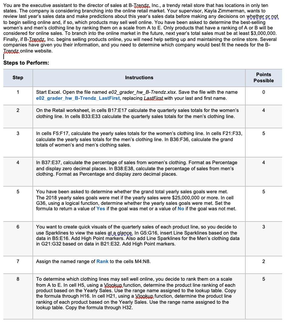
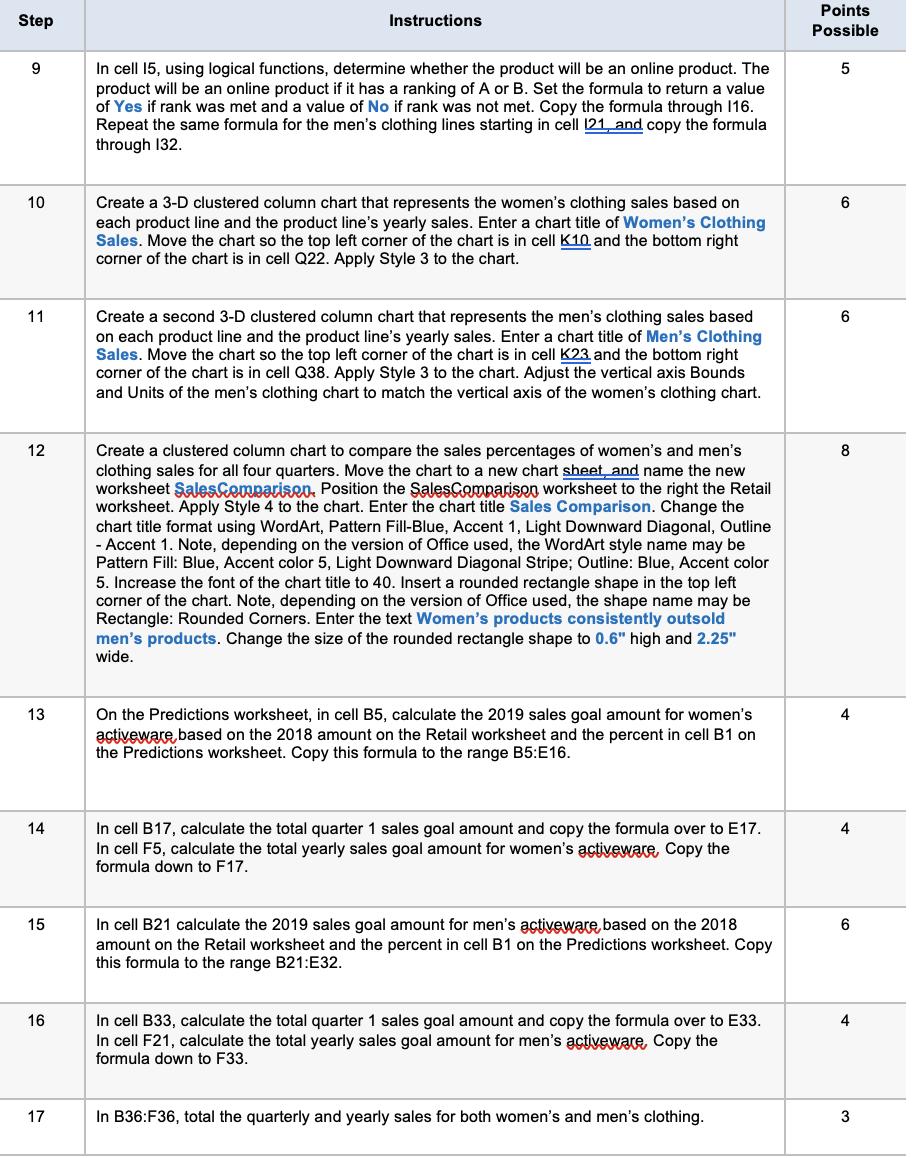
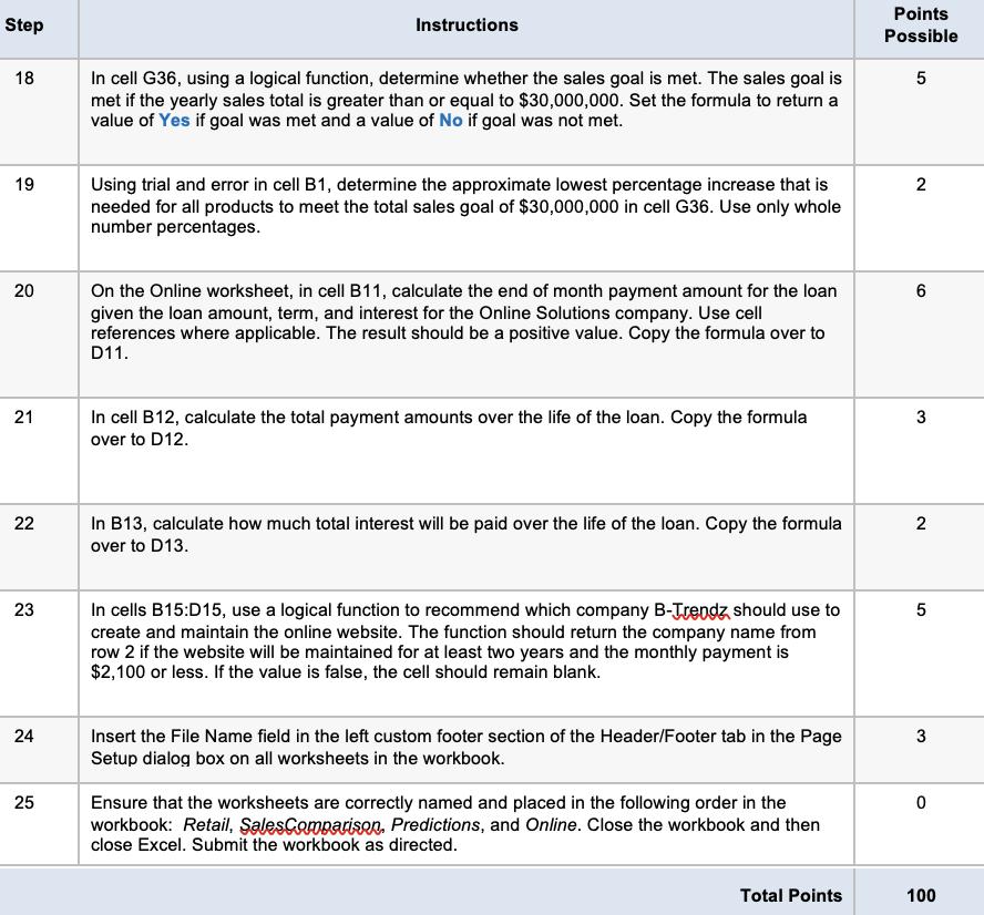
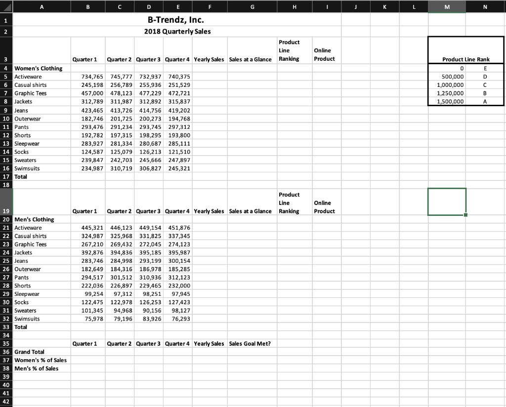
You are the executive assistant to the director of sales at B-Trendz, Inc., a trendy retail store that has locations in only ten states. The company is considering branching into the online retail market. Your supervisor, Kayla Zimmerman, wants to review last year's sales data and make predictions about this year's sales data before making any decisions on whether or not to begin selling online and, if so, which products may sell well online. You have been asked to determine the best-selling women's and men's clothing line by ranking them on a scale from A to E. Only products that have a ranking of A or B will be considered for online sales. To branch into the online market in the future, next year's total sales must be at least $3,000,000. Finally, if B-Trendz, Inc. begins selling products online, you will need help setting up and maintaining the online store. Several companies have given you their information, and you need to determine which company would best fit the needs for the B- Trendz online website. Steps to Perform: Step Instructions Points Possible 1 Start Excel. Open the file named e02_grader_hw_B-Trendz.xlsx. Save the file with the name e02 grader_hw_B-Trendz_LastFirst, replacing LastFirst with your last and first name. 0 2 On the Retail worksheet, in cells B17:E17 calculate the quarterly sales totals for the women's clothing line. In cells B33:E33 calculate the quarterly sales totals for the men's clothing line. 4 3 In cells F5:F17, calculate the yearly sales totals for the women's clothing line. In cells F21:F33, calculate the yearly sales totals for the men's clothing line. In B36:F36, calculate the grand totals of women's and men's clothing sales. 5 4 In B37:E37, calculate the percentage of sales from women's clothing. Format as Percentage and display zero decimal places. In B38:E38, calculate the percentage of sales from men's clothing. Format as Percentage and display zero decimal places. 4 5 6 You have been asked to determine whether the grand total yearly sales goals were met. The 2018 yearly sales goals were met if the yearly sales were $25,000,000 or more. In cell G36, using a logical function, determine whether the yearly sales goals were met. Set the formula to return a value of Yes if the goal was met or a value of No if the goal was not met. 5 You want to create quick visuals of the quarterly sales of each product line, so you decide to use Sparklines to view the sales at a glance. In G5:G16, insert Line Sparklines based on the data in B5:E16. Add High Point markers. Also add Line Sparklines for the Men's clothing data in G21:G32 based on data in B21:E32. Add High Point markers. 3 7 Assign the named range of Rank to the cells M4:N8. 2 8 To determine which clothing lines may sell well online, you decide to rank them on a scale from A to E. In cell H5, using a Vlookup function, determine the product line ranking of each product based on the Yearly Sales. Use the range name assigned to the lookup table. Copy the formula through H16. In cell H21, using a Vlookup function, determine the product line ranking of each product based on the Yearly Sales. Use the range name assigned to the lookup table. Copy the formula through H32. 5 Step 9 Instructions In cell 15, using logical functions, determine whether the product will be an online product. The product will be an online product if it has a ranking of A or B. Set the formula to return a value of Yes if rank was met and a value of No if rank was not met. Copy the formula through 116. Repeat the same formula for the men's clothing lines starting in cell 121 and copy the formula through 132. Points Possible 5 10 11 12 Create a 3-D clustered column chart that represents the women's clothing sales based on each product line and the product line's yearly sales. Enter a chart title of Women's Clothing Sales. Move the chart so the top left corner of the chart is in cell K10 and the bottom right corner of the chart is in cell Q22. Apply Style 3 to the chart. Create a second 3-D clustered column chart that represents the men's clothing sales based on each product line and the product line's yearly sales. Enter a chart title of Men's Clothing Sales. Move the chart so the top left corner of the chart is in cell K23 and the bottom right corner of the chart is in cell Q38. Apply Style 3 to the chart. Adjust the vertical axis Bounds and Units of the men's clothing chart to match the vertical axis of the women's clothing chart. Create a clustered column chart to compare the sales percentages of women's and men's clothing sales for all four quarters. Move the chart to a new chart sheet and name the new worksheet SalesComparison, Position the SalesComparison worksheet to the right the Retail worksheet. Apply Style 4 to the chart. Enter the chart title Sales Comparison. Change the chart title format using WordArt, Pattern Fill-Blue, Accent 1, Light Downward Diagonal, Outline - Accent 1. Note, depending on the version of Office used, the WordArt style name may be Pattern Fill: Blue, Accent color 5, Light Downward Diagonal Stripe; Outline: Blue, Accent color 5. Increase the font of the chart title to 40. Insert a rounded rectangle shape in the top left corner of the chart. Note, depending on the version of Office used, the shape name may be Rectangle: Rounded Corners. Enter the text Women's products consistently outsold men's products. Change the size of the rounded rectangle shape to 0.6" high and 2.25" wide. 6 6 8 13 On the Predictions worksheet, in cell B5, calculate the 2019 sales goal amount for women's activeware based on the 2018 amount on the Retail worksheet and the percent in cell B1 on the Predictions worksheet. Copy this formula to the range B5:E16. 4 14 In cell B17, calculate the total quarter 1 sales goal amount and copy the formula over to E17. In cell F5, calculate the total yearly sales goal amount for women's activeware, Copy the formula down to F17. 4 15 In cell B21 calculate the 2019 sales goal amount for men's activeware based on the 2018 amount on the Retail worksheet and the percent in cell B1 on the Predictions worksheet. Copy this formula to the range B21:E32. 6 16 In cell B33, calculate the total quarter 1 sales goal amount and copy the formula over to E33. In cell F21, calculate the total yearly sales goal amount for men's activeware Copy the formula down to F33. 4 17 In B36:F36, total the quarterly and yearly sales for both women's and men's clothing. 3 Step 18 Instructions In cell G36, using a logical function, determine whether the sales goal is met. The sales goal is met if the yearly sales total is greater than or equal to $30,000,000. Set the formula to return a value of Yes if goal was met and a value of No if goal was not met. Points Possible 5 19 Using trial and error in cell B1, determine the approximate lowest percentage increase that is needed for all products to meet the total sales goal of $30,000,000 in cell G36. Use only whole number percentages. 2 20 20 On the Online worksheet, in cell B11, calculate the end of month payment amount for the loan given the loan amount, term, and interest for the Online Solutions company. Use cell references where applicable. The result should be a positive value. Copy the formula over to D11. 6 221 21 In cell B12, calculate the total payment amounts over the life of the loan. Copy the formula over to D12. 3 22 22 23 In B13, calculate how much total interest will be paid over the life of the loan. Copy the formula over to D13. In cells B15:D15, use a logical function to recommend which company B-Trendz should use to create and maintain the online website. The function should return the company name from row 2 if the website will be maintained for at least two years and the monthly payment is $2,100 or less. If the value is false, the cell should remain blank. 2 5 Total Points 100 24 24 Insert the File Name field in the left custom footer section of the Header/Footer tab in the Page Setup dialog box on all worksheets in the workbook. 3 25 25 Ensure that the worksheets are correctly named and placed in the following order in the workbook: Retail, SalesComparison, Predictions, and Online. Close the workbook and then close Excel. Submit the workbook as directed. 0 E B-Trendz, Inc. A B C D 1 2 F G H J K L M N 2018 Quarterly Sales Product Line Online 3 4 Women's Clothing 5 Activeware 6 Casual shirts 7 Graphic Tees 8 Jackets 9 Jeans 10 Outerwear 11 Pants 12 Shorts 13 Sleepwear 14 Socks 15 Sweaters 16 Swimsuits 17 Total 18 Quarter 1 Quarter 2 Quarter 3 Quarter 4 Yearly Sales Sales at a Glance Ranking Product 734,765 745,777 732,937 740,375 245,198 256,789 255,936 251,529 457,000 478,123 477,229 472,721 312,789 311,987 312,892 315,837 423,465 413,726 414,756 419,202 182,746 201,725 200,273 194,768 293,476 291,234 293,745 297,312 192,782 197,315 198,295 193,800 283,927 281,334 280,687 285,111 124,587 125,079 126,213 121,510 239,847 242,703 245,666 247,897 234,987 310,719 306,827 245,321 Product Line Online 19 Quarter 1 Quarter 2 Quarter 3 Quarter 4 Yearly Sales Sales at a Glance Ranking Product 20 Men's Clothing 445,321 446,123 449,154 451,876 324,987 325,968 331,825 337,345 21 Activeware 22 Casual shirts 23 Graphic Tees 24 Jackets 25 Jeans 26 Outerwear 27 Pants 28 Shorts 29 Sleepwear 30 Socks 31 Sweaters 32 Swimsuits 267,210 269,432 272,045 274,123 392,876 394,836 395,185 395,987 283,746 284,998 293,199 300,154 182,649 184,316 186,978 185,285 294,517 301,512 310,936 312,123 222,036 226,897 229,465 232,000 99,254 97,312 98,251 97,945 122,475 122,978 126,253 127,423 101,345 94,968 90,156 98,127 75,978 79,196 83,926 76,293 33 Total 34 35 36 Grand Total 37 Women's % of Sales 38 Men's % of Sales Quarter 1 Quarter 2 Quarter 3 Quarter 4 Yearly Sales Sales Goal Met? 39 40 41 42 Product Line Rank 0 E 500,000 D 1,000,000 1,250,000 1,500,000 B A