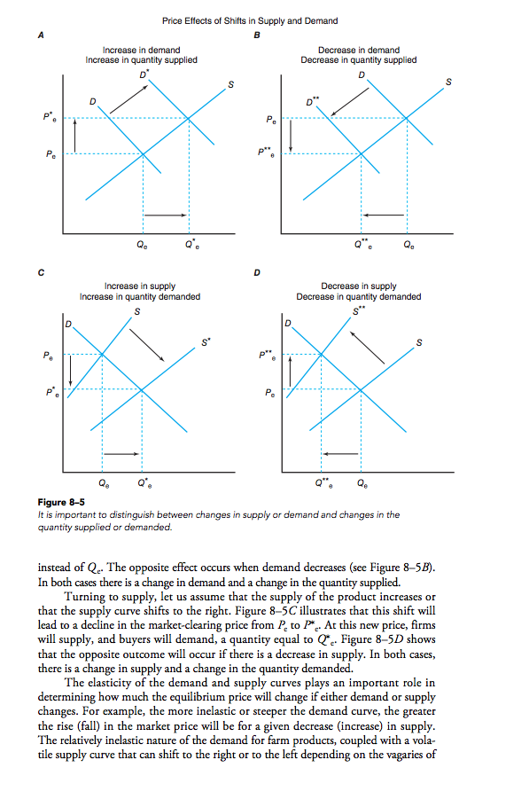
you will be given a scenario that would cause a shift in supply or demand. You will also be required to show how price/quantity changes as Supply and Demand shifts. You can use Microsoft Word or Excel to draw your graphs. Each graph should have a title, a label for each axis and you must show the direction of the shift using an arrow. Each line should be labeled also ( Supply or Demand). For each graph you will need both Supply and Demand lines. Before starting this assignment, you might want to refer to Chapter 8: Market Equilibrium, Page 140.

1. Create a graph using supply and demand lines to show how prices and quantity would be affected by an economic downturn such as a recession. (A recession causes a decrease in demand).

2. Create a graph using supply and demand lines to show how prices and quantity would be affected by a decrease in the price of a substitute.

3. Create a graph using supply and demand lines to show how prices and quantity would be affected by a "bumper crop" year.

4. Create a graph using supply and demand lines to show how prices and quantity would be affected in agriculture by an increase in production costs.

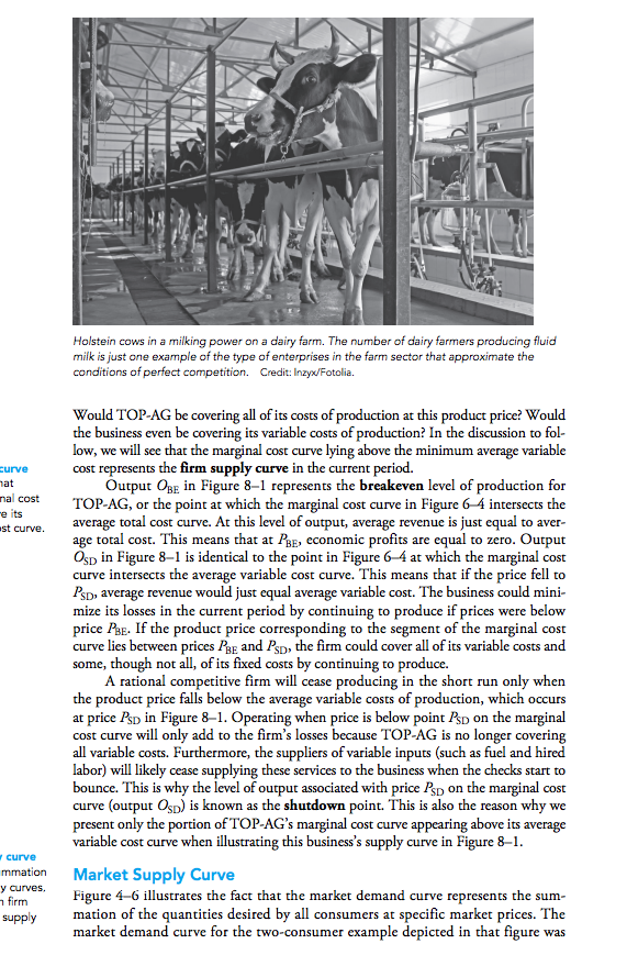
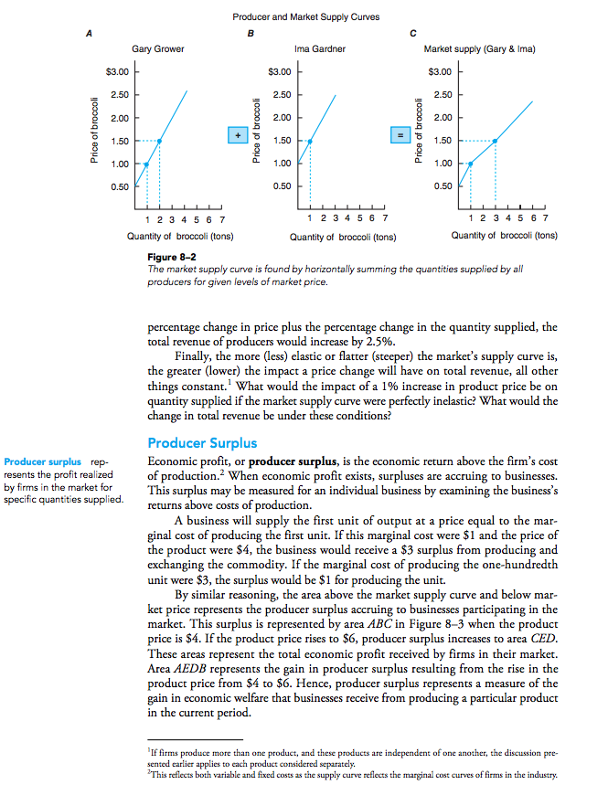
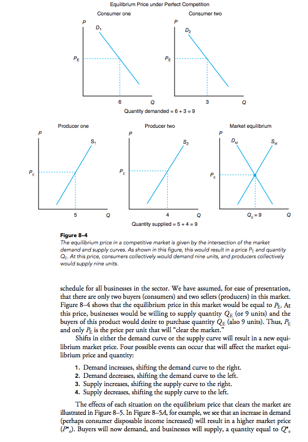
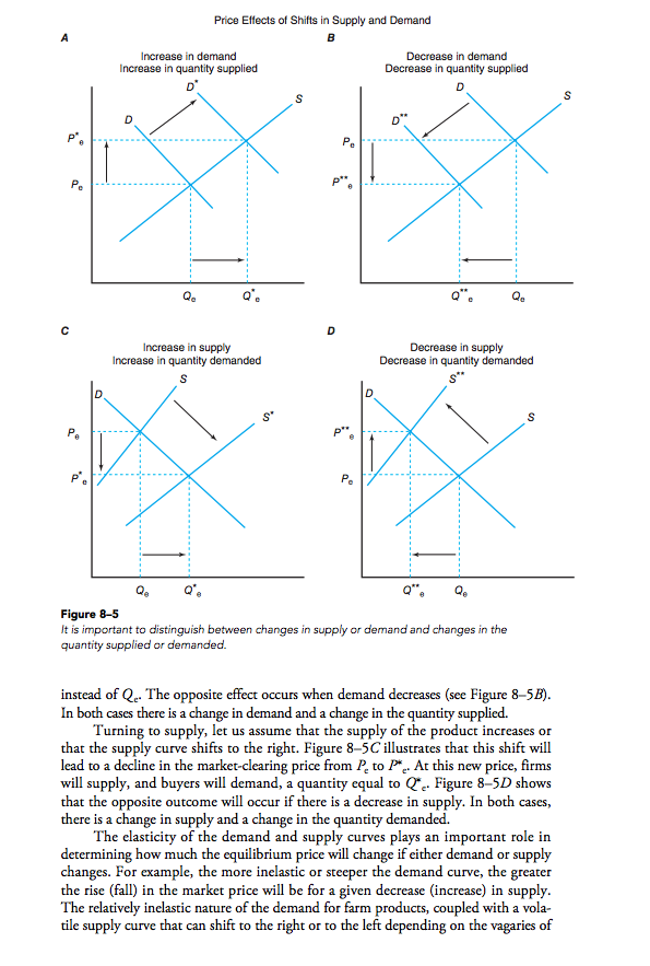
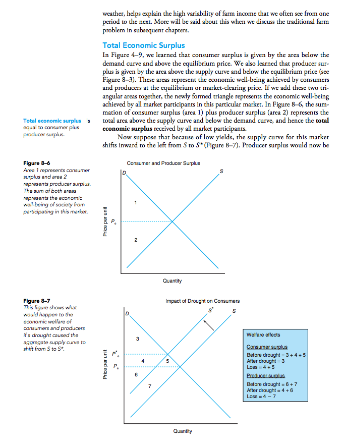
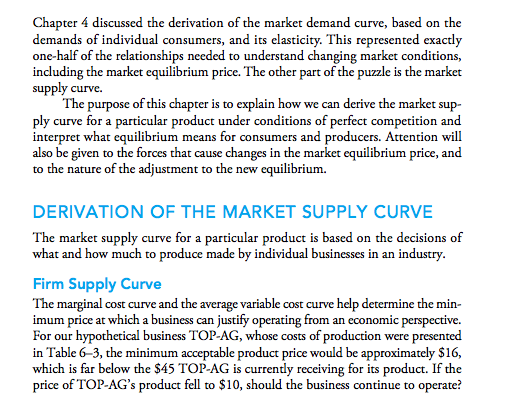
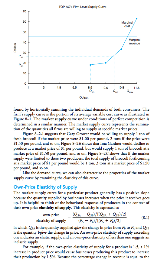
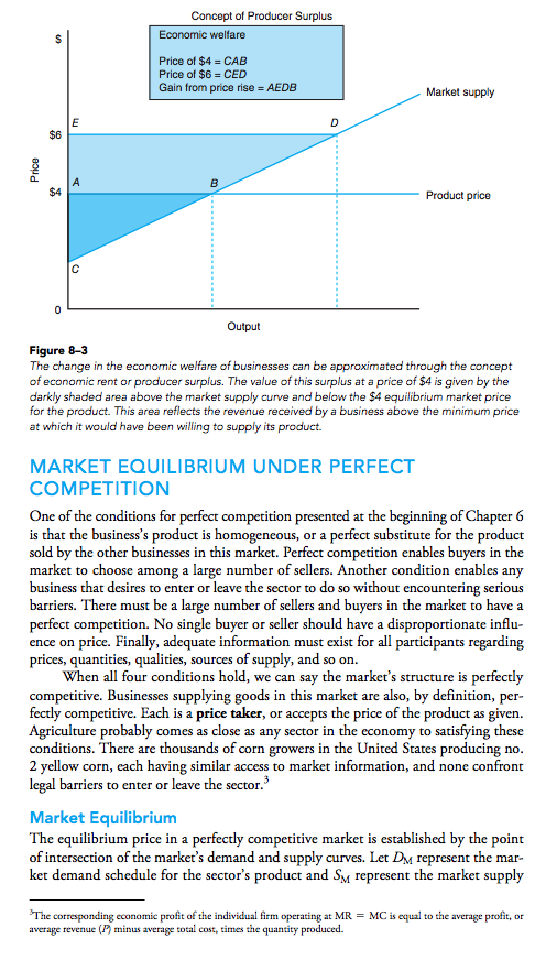
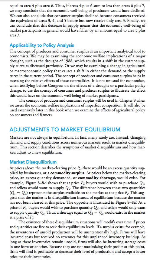
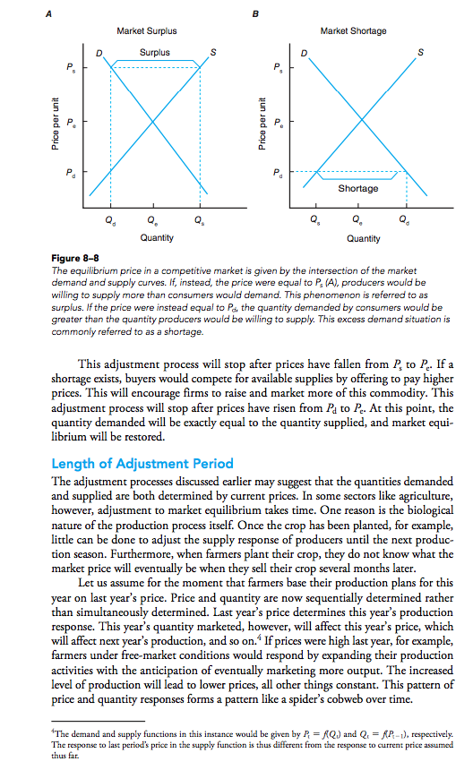
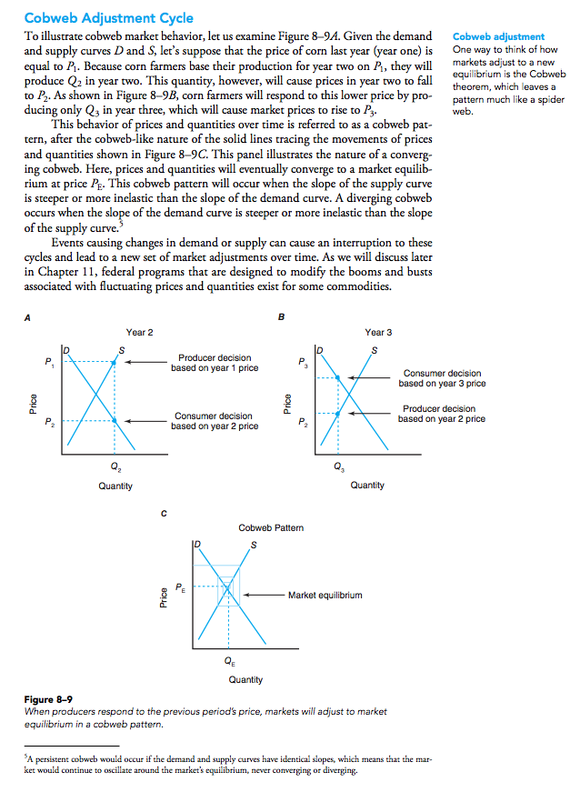
Chapter 4 discussed the derivation of the market demand curve, based on the demands of individual consumers, and its elasticity. This represented exactly one-half of the relationships needed to understand changing market conditions, including the market equilibrium price. The other part of the puzzle is the market supply curve. The purpose of this chapter is to explain how we can derive the market sup- ply curve for a particular product under conditions of perfect competition and interpret what equilibrium means for consumers and producers. Attention will also be given to the forces that cause changes in the market equilibrium price, and to the nature of the adjustment to the new equilibrium. DERIVATION OF THE MARKET SUPPLY CURVE The market supply curve for a particular product is based on the decisions of what and how much to produce made by individual businesses in an industry. Firm Supply Curve The marginal cost curve and the average variable cost curve help determine the min- imum price at which a business can justify operating from an economic perspective. For our hypothetical business TOP-AG, whose costs of production were presented in Table 6-3, the minimum acceptable product price would be approximately $16, which is far below the $45 TOP-AG is currently receiving for its product. If the price of TOP-AG's product fell to $10, should the business continue to operate?Holstein cows in a milking power on a dairy farm. The number of dairy farmers producing fluid milk is just one example of the type of enterprises in the farm sector that approximate the conditions of perfect competition. Credit: Inzyx/Fotolia. Would TOP-AG be covering all of its costs of production at this product price? Would the business even be covering its variable costs of production? In the discussion to fol- low, we will see that the marginal cost curve lying above the minimum average variable curve cost represents the firm supply curve in the current period. iat Output OBE in Figure 8-1 represents the breakeven level of production for na cost e its TOP-AG, or the point at which the marginal cost curve in Figure 6 4 intersects the st curve. average total cost curve. At this level of output, average revenue is just equal to aver- age total cost. This means that at BE, economic profits are equal to zero. Output On in Figure 8-1 is identical to the point in Figure 6-4 at which the marginal cost curve intersects the average variable cost curve. This means that if the price fell to P'sD average revenue would just equal average variable cost. The business could mini- mize its losses in the current period by continuing to produce if prices were below price PRE. If the product price corresponding to the segment of the marginal cost curve lies between prices BE and Pep, the firm could cover all of its variable costs and some, though not all, of its fixed costs by continuing to produce. A rational competitive firm will cease producing in the short run only when the product price falls below the average variable costs of production, which occurs at price Pop in Figure 8-1. Operating when price is below point Asp on the marginal cost curve will only add to the firm's losses because TOP-AG is no longer covering all variable costs. Furthermore, the suppliers of variable inputs (such as fuel and hired labor) will likely cease supplying these services to the business when the checks start to bounce. This is why the level of output associated with price P'sp on the marginal cost curve (output Op) is known as the shutdown point. This is also the reason why we present only the portion of TOP-AG's marginal cost curve appearing above its average variable cost curve when illustrating this business's supply curve in Figure 8-1. curve mmation Market Supply Curve y curves. 1 firm Figure 4-6 illustrates the fact that the market demand curve represents the sum- supply mation of the quantities desired by all consumers at specific market prices. The market demand curve for the two-consumer example depicted in that figure wasTOP-AG's Firm-Level Supply Curve 70 60 Marginal cost 50 Marginal 40 : revenue Dollars 30 20 10 3 4.8 6.5 8.5 9.6 10.8 11.6 Output found by horizontally summing the individual demands of both consumers. The firm's supply curve is the portion of its average variable cost curve as illustrated in Figure 8-1. The market supply curve under conditions of perfect competition is determined in a similar manner. The market supply curve represents the summa- tion of the quantities all firms are willing to supply at specific market prices. Figure 8-24 suggests that Gary Grower would be willing to supply 1 ton of fresh broccoli if the market price were $1.00 per pound, 2 tons if the price were $1.50 per pound, and so on. Figure 8-2B shows that Ima Gardner would decline to produce at a market price of $1 per pound, but would supply 1 ton of broccoli at a market price of $1.50 per pound, and so on. Figure 8-2C shows that if the market supply were limited to these two producers, the total supply of broccoli forthcoming at a market price of $1 per pound would be 1 ton, 3 tons at a market price of $1.50 per pound, and so on. Like the demand curve, we can also characterize the properties of the market supply curve by examining the elasticity of this curve. Own-Price Elasticity of Supply The market supply curve for a particular product generally has a positive slope because the quantity supplied by businesses increases when the price it receives goes up. It is helpful to think of the behavioral response of producers in the context of their own-price elasticity of supply. This elasticity is expressed as own-price (QSA - QSB) / [(QSA + QSB)/2] (8.1) elasticity of supply (PA - P) / [(PA + PB) /2] in which QsA is the quantity supplied after the change in price from P to PA and QB is the quantity before the change in price. An own-price elasticity of supply exceeding one indicates an elastic supply, and an own-price elasticity of less than one suggests an inelastic supply. For example, if the own-price elasticity of supply for a product is 1.5, a 1% increase in product price would cause businesses producing this product to increase their production by 1.5%. Because the percentage change in revenue is equal to theProducer and Market Supply Curves A B C Gary Grower Ima Gardner Market supply (Gary & Ima) $3.00 $3.00 $3.00 2.50 2.50 2.50 2.00 2.00 2.00 Price of broccoli Price of broccoli Price of broccoli 1.50 + 1.50 = 1.50 1.00 1.00 1.00 0.50 0.50 0.5 1 2 3 4 5 6 7 1 2 3 4 5 6 7 1 2 3 4 5 6 7 Quantity of broccoli (tons) Quantity of broccoli (tons) Quantity of broccoli (tons) Figure 8-2 The market supply curve is found by horizontally summing the quantities supplied by all producers for given levels of market price. percentage change in price plus the percentage change in the quantity supplied, the total revenue of producers would increase by 2.5% Finally, the more (less) elastic or flatter (steeper) the market's supply curve is, the greater (lower) the impact a price change will have on total revenue, all other things constant.' What would the impact of a 1% increase in product price be on quantity supplied if the market supply curve were perfectly inelastic? What would the change in total revenue be under these conditions? Producer Surplus Producer surplus rep- Economic profit, or producer surplus, is the economic return above the firm's cost resents the profit realized of production. When economic profit exists, surpluses are accruing to businesses by firms in the market for specific quantities supplied. This surplus may be measured for an individual business by examining the business's returns above costs of production. A business will supply the first unit of output at a price equal to the mar- ginal cost of producing the first unit. If this marginal cost were $1 and the price of the product were $4, the business would receive a $3 surplus from producing and exchanging the commodity. If the marginal cost of producing the one-hundredth unit were $3, the surplus would be $1 for producing the unit. By similar reasoning, the area above the market supply curve and below mar- ket price represents the producer surplus accruing to businesses participating in the market. This surplus is represented by area ABC in Figure 8-3 when the product price is $4. If the product price rises to $6, producer surplus increases to area CED. These areas represent the total economic profit received by firms in their market. Area AEDB represents the gain in producer surplus resulting from the rise in the product price from $4 to $6. Hence, producer surplus represents a measure of the gain in economic welfare that businesses receive from producing a particular product in the current period. "If firms produce more than one product, and these products are independent of one another, the discussion pre- sented earlier applies to each product considered separately. "This reflects both variable and fixed costs as the supply curve reflects the marginal cost curves of firms in the industry.Concept of Producer Surplus Economic welfare Price of $4 = CAB Price of $6 = CED Gain from price rise = AEDB Market supply D $6 Price A $4 Product price C Output Figure 8-3 The change in the economic welfare of businesses can be approximated through the concept of economic rent or producer surplus. The value of this surplus at a price of $4 is given by the darkly shaded area above the market supply curve and below the $4 equilibrium market price for the product. This area reflects the revenue received by a business above the minimum price at which it would have been willing to supply its product. MARKET EQUILIBRIUM UNDER PERFECT COMPETITION One of the conditions for perfect competition presented at the beginning of Chapter 6 is that the business's product is homogeneous, or a perfect substitute for the product sold by the other businesses in this market. Perfect competition enables buyers in the market to choose among a large number of sellers. Another condition enables any business that desires to enter or leave the sector to do so without encountering serious barriers. There must be a large number of sellers and buyers in the market to have a perfect competition. No single buyer or seller should have a disproportionate influ- ence on price. Finally, adequate information must exist for all participants regarding prices, quantities, qualities, sources of supply, and so on. When all four conditions hold, we can say the market's structure is perfectly competitive. Businesses supplying goods in this market are also, by definition, per- fectly competitive. Each is a price taker, or accepts the price of the product as given. Agriculture probably comes as close as any sector in the economy to satisfying these conditions. There are thousands of corn growers in the United States producing no. 2 yellow corn, each having similar access to market information, and none confront legal barriers to enter or leave the sector." Market Equilibrium The equilibrium price in a perfectly competitive market is established by the point of intersection of the market's demand and supply curves. Let Dy represent the mar- ket demand schedule for the sector's product and SM represent the market supply The corresponding economic profit of the individual firm operating at MR = MC is equal to the average profit, or average revenue (") minus average total cost, times the quantity produced.Equilibrium Price under Perfect Competition Consumer one Consumer two PE PE 6 3 Q Quantity demanded = 6 + 3 =9 Producer one Producer two Market equilibrium P S2 PE PF PE 5 QE =9 Quantity supplied = 5 + 4 = 9 Figure 8-4 The equilibrium price in a competitive market is given by the intersection of the market demand and supply curves. As shown in this figure, this would result in a price PE and quantity Q:. At this price, consumers collectively would demand nine units, and producers collectively would supply nine units. schedule for all businesses in the sector. We have assumed, for ease of presentation, that there are only two buyers (consumers) and two sellers (producers) in this market Figure 8-4 shows that the equilibrium price in this market would be equal to PE. At this price, businesses would be willing to supply quantity OF (or 9 units) and the buyers of this product would desire to purchase quantity QE (also 9 units). Thus, PE and only P: is the price per unit that will "clear the market." Shifts in either the demand curve or the supply curve will result in a new equi- librium market price. Four possible events can occur that will affect the market equi- librium price and quantity: 1. Demand increases, shifting the demand curve to the right. 2. Demand decreases, shifting the demand curve to the left. 3. Supply increases, shifting the supply curve to the right. 4. Supply decreases, shifting the supply curve to the left. The effects of each situation on the equilibrium price that clears the market are illustrated in Figure 8 5. In Figure 8-54, for example, we see that an increase in demand (perhaps consumer disposable income increased) will result in a higher market price (P*). Buyers will now demand, and businesses will supply, a quantity equal to QPrice Effects of Shifts in Supply and Demand A B Increase in demand Decrease in demand Increase in quantity supplied Decrease in quantity supplied S S P" P Qe Q e C D Increase in supply Decrease in supply Increase in quantity demanded Decrease in quantity demanded PA Qa Qe Figure 8-5 It is important to distinguish between changes in supply or demand and changes in the quantity supplied or demanded. instead of Q: The opposite effect occurs when demand decreases (see Figure 8-58). In both cases there is a change in demand and a change in the quantity supplied Turning to supply, let us assume that the supply of the product increases or that the supply curve shifts to the right. Figure 8-5C illustrates that this shift will lead to a decline in the market-clearing price from P, to *. At this new price, firms will supply, and buyers will demand, a quantity equal to Q". Figure 8-5D shows that the opposite outcome will occur if there is a decrease in supply. In both cases, there is a change in supply and a change in the quantity demanded. The elasticity of the demand and supply curves plays an important role in determining how much the equilibrium price will change if either demand or supply changes. For example, the more inelastic or steeper the demand curve, the greater the rise (fall) in the market price will be for a given decrease (increase) in supply. The relatively inelastic nature of the demand for farm products, coupled with a vola- tile supply curve that can shift to the right or to the left depending on the vagaries ofPrice Effects of Shifts in Supply and Demand A Increase in demand Decrease in demand Increase in quantity supplied Decrease in quantity supplied D PA P Qe Q - C D rease in Decrease in supply Increase in quantity demanded Decrease in quantity demanded P Qe Figure 8-5 It is important to distinguish between changes in supply or demand and changes in the quantity supplied or demanded. instead of Q- The opposite effect occurs when demand decreases (see Figure 8-58). In both cases there is a change in demand and a change in the quantity supplied Turning to supply, let us assume that the supply of the product increases or that the supply curve shifts to the right. Figure 8-5C illustrates that this shift will lead to a decline in the market-clearing price from P, to P. At this new price, firms will supply, and buyers will demand, a quantity equal to Q". Figure 8-5D shows that the opposite outcome will occur if there is a decrease in supply. In both cases, there is a change in supply and a change in the quantity demanded. The elasticity of the demand and supply curves plays an important role in determining how much the equilibrium price will change if either demand or supply changes. For example, the more inelastic or steeper the demand curve, the greater the rise (fall) in the market price will be for a given decrease (increase) in supply. The relatively inelastic nature of the demand for farm products, coupled with a vola- tile supply curve that can shift to the right or to the left depending on the vagaries ofweather, helps explain the high variability of farm income that we often see from one period to the next. More will be said about this when we discuss the traditional farm problem in subsequent chapters. Total Economic Surplus In Figure 4-9, we learned that consumer surplus is given by the area below the demand curve and above the equilibrium price. We also learned that producer sur- plus is given by the area above the supply curve and below the equilibrium price (see Figure 8-3). These areas represent the economic well-being achieved by consumers and producers at the equilibrium or market-clearing price. If we add these two tri- angular areas together, the newly formed triangle represents the economic well-being achieved by all market participants in this particular market. In Figure 8-6, the sum- mation of consumer surplus (area 1) plus producer surplus (area 2) represents the Total economic surplus is total area above the supply curve and below the demand curve, and hence the total equal to consumer plus economic surplus received by all market participants. producer surplus. Now suppose that because of low yields, the supply curve for this market shifts inward to the left from $ to S* (Figure 8-7). Producer surplus would now be Figure 8-6 Consumer and Producer Surplus Area 1 represents consumer surplus and area 2 represents producer surplus. The sum of both areas represents the economic well-being of society from participating in this market. Price per unit Quantity Figure 8-7 Impact of Drought on Consumers This figure shows what would happen to the economic welfare of consumers and producers if a drought caused the Welfare effects aggregate supply curve to shift from S to 5*. Consumer surplus P . Before drought = 3 + 4 +5 15 After drought = 3 Price per unit P. Loss = 4 +5 Producer surplus Before drought = 6 + 7 After drought = 4 + 6 Loss = 4 - 7 Quantityequal to area 4 plus area 6. Thus, if areas 4 plus 6 sum to less than areas 6 plus 7, we may conclude that the economic well-being of producers would have declined. We can also conclude that consumer surplus declined because consumers received the equivalent of areas 3, 4, and 5 before but now receive only area 3. Finally, we can conclude that this decrease in supply means that the economic well-being of market participants in general would have fallen by an amount equal to area 5 plus area 7. Applicability to Policy Analysis The concept of producer and consumer surplus is an important analytical tool to economists. We may be examining the economic welfare implications of a major drought, such as the drought of 1988, which results in a shift in the current sup- ply curve as discussed previously. Or we may be examining a change in agricultural or macroeconomic policy that causes a shift in either the demand or the supply curve in the current period. The concept of producer and consumer surplus helps in assessing the relative effects of these externalities. It is not unusual for economists, when testifying before Congress on the effects of a drought or a particular policy change, to use the concept of consumer and producer surplus to illustrate the effect this would have on the economic well-being of market participants. The concept of producer and consumer surplus will be used in Chapter 9 when we assess the economic welfare implications of imperfect competition. It will also be used extensively later in this book when we examine the effects of agricultural policy on consumers and farmers. ADJUSTMENTS TO MARKET EQUILIBRIUM Markets are not always in equilibrium. In fact, many rarely are. Instead, changing demand and supply conditions across numerous markets result in market disequilib rium. This section describes the symptoms of market disequilibrium and how mar- kets adjust to a new equilibrium. Market Disequilibrium At prices above the market-clearing price ,, there would be an excess quantity sup- plied by businesses, or a commodity surplus. At prices below the market-clearing price, an excess quantity demanded, or commodity shortage, would exist. For example, Figure 8 84 shows that at price , buyers would wish to purchase Qad and sellers would want to supply Q,. The difference between these two quantities (Q, - Q ) represents the surplus available on the market at the price P. This sug- gests that the market is in disequilibrium instead of equilibrium because the market has not been cleared at this price. The opposite is illustrated in Figure 8-8B. At a price of Pa, buyers would wish to purchase quantity Qa, and sellers would only want to supply quantity Q.. Thus, a shortage equal to Q1 - Q, would exist in the market at a price of Pa. The existence of these disequilibrium situations will modify over time if prices and quantities are free to seek their equilibrium levels. If a surplus exists, for example, the inventories of unsold production will be unintentionally high. Firms will have incurred costs but received no revenues for this unplanned inventory buildup. As long as these inventories remain unsold, firms will also be incurring storage costs in one form or another. Because they are not maximizing their profits at this point, firms will find it profitable to decrease their level of production and accept a lower price for their inventories.B Market Surplus Market Shortage Surplus S Price per unit P Price per unit P P PA Shortage Q. Quantity Quantity Figure 8-8 The equilibrium price in a competitive market is given by the intersection of the market demand and supply curves. If, instead, the price were equal to P, (A), producers would be willing to supply more than consumers would demand. This phenomenon is referred to as surplus. If the price were instead equal to Pa, the quantity demanded by consumers would be greater than the quantity producers would be willing to supply. This excess demand situation is commonly referred to as a shortage. This adjustment process will stop after prices have fallen from P, to P. If a shortage exists, buyers would compete for available supplies by offering to pay higher prices. This will encourage firms to raise and market more of this commodity. This adjustment process will stop after prices have risen from Pa to P. At this point, the quantity demanded will be exactly equal to the quantity supplied, and market equi- librium will be restored. Length of Adjustment Period The adjustment processes discussed earlier may suggest that the quantities demanded and supplied are both determined by current prices. In some sectors like agriculture, however, adjustment to market equilibrium takes time. One reason is the biological nature of the production process itself. Once the crop has been planted, for example, little can be done to adjust the supply response of producers until the next produc- tion season. Furthermore, when farmers plant their crop, they do not know what the market price will eventually be when they sell their crop several months later. Let us assume for the moment that farmers base their production plans for this year on last year's price. Price and quantity are now sequentially determined rather than simultaneously determined. Last year's price determines this year's production response. This year's quantity marketed, however, will affect this year's price, which will affect next year's production, and so on.* If prices were high last year, for example, farmers under free-market conditions would respond by expanding their production activities with the anticipation of eventually marketing more output. The increased level of production will lead to lower prices, all other things constant. This pattern of price and quantity responses forms a pattern like a spider's cobweb over time. "The demand and supply functions in this instance would be given by R = (Q) and Q, = AR-1), respectively. The response to last period's price in the supply function is thus different from the response to current price assumed thus far.Cobweb Adjustment Cycle To illustrate cobweb market behavior, let us examine Figure 8-94. Given the demand Cobweb adjustment and supply curves D and S, let's suppose that the price of corn last year (year one) is One way to think of how equal to Pi. Because corn farmers base their production for year two on A, they will markets adjust to a new produce Q2 in year two. This quantity, however, will cause prices in year two to fall equilibrium is the Cobweb theorem, which leaves a to P. As shown in Figure 8-98, corn farmers will respond to this lower price by pro- pattern much like a spider ducing only Q3 in year three, which will cause market prices to rise to '3. web. This behavior of prices and quantities over time is referred to as a cobweb pat- tern, after the cobweb-like nature of the solid lines tracing the movements of prices and quantities shown in Figure 8-9C. This panel illustrates the nature of a converg ing cobweb. Here, prices and quantities will eventually converge to a market equilib rium at price PE. This cobweb pattern will occur when the slope of the supply curve is steeper or more inelastic than the slope of the demand curve. A diverging cobweb occurs when the slope of the demand curve is steeper or more inelastic than the slope of the supply curve.' Events causing changes in demand or supply can cause an interruption to these cycles and lead to a new set of market adjustments over time. As we will discuss later in Chapter 11, federal programs that are designed to modify the booms and busts associated with fluctuating prices and quantities exist for some commodities. A B Year 2 Year 3 S S Producer decision based on year 1 price P Consumer decision based on year 3 price Price Price Producer decision Consumer decision based on year 2 price based on year 2 price P. Q, Quantity Quantity C Cobweb Pattern PE Price X- Market equilibrium QE Quantity Figure 8-9 When producers respond to the previous period's price, markets will adjust to market equilibrium in a cobweb pattern. 'A persistent cobweb would occur if the demand and supply curves have identical slopes, which means that the mar- ket would continue to oscillate around the market's equilibrium, never converging or diverging