Question
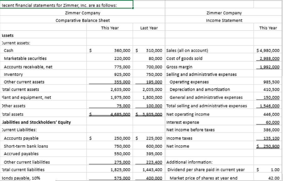
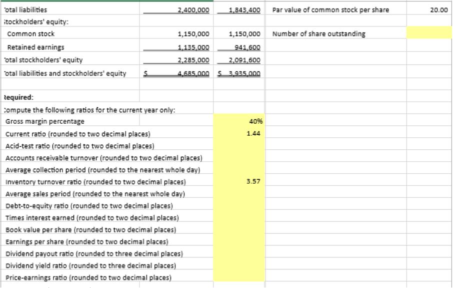
Zimmer, Inc. has provided its recent financial statements.The Controller has asked you to use this information to compute and interpret financial ratios that managers are

Zimmer, Inc. has provided its recent financial statements.The Controller has asked you to use this information to compute and interpret financial ratios that managers are going to use to assess liquidity and use for asset and debt management purposes.Use the information included in the Excel Simulation and the Excel functions described below to complete the task.
EXCEL functions:
- Cell Reference:Allows you to refer to data from another cell in the worksheet.From the Excel Simulation below, if in a blank cell, "=B7" was entered, the formula would output the result from cell B7, or 360,000 in this example.
- Basic Math functions:Allows you to use the basic math symbols to perform mathematical functions.You can use the following keys:+ (plus sign to add), - (minus sign to subtract), * (asterisk sign to multiply), and / (forward slash to divide).From the Excel Simulation below, if in a blank cell "=C13+C14" was entered, the formula would add the values from those cells and output the result, or 1,900,000 in this example.If using the other math symbols the result would output an appropriate answer for its function.
- ROUND function:Allows you to round a number or result of a formula calculation to a specific number of digits.The syntax of the ROUND function is "=ROUND(number,num_digits)" and returns the result of your formula rounded to a particular number of digits.The number argument can be a cell reference to a number or a formula itself that results in a number.The num_digits argument is the number of digits you want to round.The num_digits value rounds based on basis mathematical rounding rules, where anything below 5 will round down and anything 5 and above rounds up.Also, the num_digits value should be a positive value to round to any number of decimal places, while a negative value would round to the left of the decimal place, and a zero would round to the nearest whole number.If the value 1,253.5693 was entered in cell A1, it can be used in the ROUND function as the number reference.In this example, if the value in cell A1 should be rounded to 2 decimal places, in a new cell the function would be written as "=ROUND(A1,2)" and would result in as 1,253.57 in this example.If the number in cell A1 should be rounded to the nearest hundred place, in a new cell the function would be written as "=ROUND(A1,-2)" and would result in 1,300 in this example.
Hints:
- Each yellow cell must contain a formula that can calculate the required ratio (you can NOT input the ratio itself). Make sure you start each formula with the "=" sign. For example, gross margin percentage is calculated by dividing the gross margin by total sales, so input the formula "=F9/F7".You could also input the equals sign to start your formula and then click on the F9 cell then input the divide sign and then click on the F7 cell.
- Make sure you follow the rounding instructions. For example, the debt to equity ratio is to be rounded to two decimals using the formula "=ROUND(B24/B28,2)".If you are rounding to the nearest whole number, you are rounding to zero decimals.For example,the average collection period is roundedto the nearest whole day, so input "=ROUND(365/C36,0)".
- Checkyour formulasand make sure that you are grouping numbersand/or variables together with parentheses as needed; remember the order of operations concept from algebra.Some of thecell formulas will include several setsof parentheses so make sure that you open and close each set. There should be the same number of"(" and ")".For example, the formula for theinventory turnoverratio is =ROUND(F8/((B10+C10)/2),2). You're welcome :) for that one.Also, notice how the average inventory balance is calculated in the formula for the inventory turnover ratio.You addthe current and prior yearbalances together and divide by two as follows:((current year cell+prior year cell) /2).
You haveFIVE attempts for eachCELL andONE submission. After you input the formula in the cell and hit enter, the system will say CORRECT in green or INCORRECT in red (that is one attempt).Caution - The system may also count an attempt if you click on a cell and start the formula but then you click outside the cell without it being a proper reference in aformula.


Step by Step Solution
There are 3 Steps involved in it
Step: 1

Get Instant Access to Expert-Tailored Solutions
See step-by-step solutions with expert insights and AI powered tools for academic success
Step: 2

Step: 3

Ace Your Homework with AI
Get the answers you need in no time with our AI-driven, step-by-step assistance
Get Started


