Question Answers

Textbooks

Find textbooks, questions and answers

Oops, something went wrong!

Change your search query and then try again

Result Not Found

Books FREE
Study Help
Hire a Tutor
AI Tutor
AI Flashcards FREE

Search
Sign In
Register

study help
computer science
machine learning

A First Course In Machine Learning 2nd Edition Simon Rogers , Mark Girolam - Solutions

For some one-dimensional input data, construct a GP RBF covariance matrix. Use Gibbs sampling to sample functions from this GP prior (samples from a GP prior are just samples from a multivariate
Use Metropolis-Hastings instead of Gibbs sampling to sample from the GP classification model. Note that you will no longer need to perform the auxiliary variable trick. Compare the predictions with
Using the provided code for performing Gibbs sampling for binary GP classification, compute the \(\hat{R}\) value for one of the training latent function values. How many samples need to be drawn
For the same GP model as in Exercise 9.3 , compute the autocorrelation of one of the training latent function values. How much thinning would be required to obtain independent samples?Data from
Generate a regression dataset by sampling a function from a GP prior and then adding some noise. Use ABC to sample from the posterior. Each sample should be generated by first sampling from the GP
For the mixture model where each component is a one-dimensional Gaussian with variance 1 , show that the conditional distribution for the mean of the \(k\) th mixture component is that given by
Implement the Gibbs sampler for the mixture model. Compute \(\hat{R}\) and the autocorrelation of the component means \(\mu_{k}\). How many samples are required for convergence? How much should the
Marginalise the Gaussian mean from the Gibbs sampler to give a conditional distribution for \(z_{n k}\) conditioned only on the other assignments and the prior parameters \(\left(\mu_{0},
Implement the collapsed Gibbs sampler for the Gaussian mixture model. At each iteration in the sampler, sample the means \(\mu_{k}\) even though they are not needed (sample them from the posterior
Implement a sampler that samples from the Chinese restaurant process. Repeatedly resample assignment of customers to tables and plot a histogram over the number of tables. Investigate how the
Write some code that will sample from a Dirichlet process. The code should store all previous samples and then copy previous samples or draw new samples from the base. Experiment with different base
Using the MATLAB script provided (MATLAB script: hdp.m), experiment with setting the values of the concentration parameters for the top level DP \((\alpha)\) and the lower DPs \(\left(\gamma_{1},
Derive a Gibbs sampling scheme for inference in the Hierarchical Dirichlet process. Assume that the base distribution is Gaussian \(\left(H=\mathcal{N}\left(\mu_{0}, \sigma_{0}^{2}\right)\right)\)
Derive the collapsed Gibbs sampler for LDA given in Equation 10.13 .Data from Equation 10.13 = k|xni = w,...) x (Ck+k) P(zni = kani Vkw + Tw w' Vkw' + Yw'
Write some code to sample from a GP prior. In particular, define some onedimensional input points ( \(x\) ), compute the covariance matrix by computing the covariance function at all pairs of points
Use a numerical optimisation routine to find the values of \(\sigma^{2}\) and \(\gamma\) that maximise the marginal likelihood for GP regression using an RBF covariance matrix (with \(\alpha=1\) ).
For some one-dimensional input data ( \(x\) ), generate a real-valued latent function using a GP prior with an RBF covariance function. For each value, sample a random integer from a Poisson
Use Metropolis-Hastings to perform inference in the binary GP classifier. The MH sampler should repeatedly resample values of \(\mathbf{f}\). For each sample, do a noise-free regression to compute
Given the expression for the area of a circle, \(A=\pi r^{2}\), and using only uniformly distributed random variates, devise a sampling approach for computing \(\pi\).
Rearrange the logistic function\[P\left(T_{\text {new }}=1 \mid \mathbf{x}_{\text {new }}, \widehat{\mathbf{w}}\right)=\frac{1}{1+\exp \left(-\widehat{\mathbf{w}}^{\top} \mathbf{x}_{\text {new
Assume that we observe \(N\) vectors of attributes, \(\mathbf{x}_{1}, \ldots, \mathbf{x}_{N}\) and associated integer counts \(t_{1}, \ldots, t_{N}\). A Poisson likelihood would be
Assuming \(\boldsymbol{\Sigma}_{c}=\mathbf{I}\) for all classes, compute the posterior density \(p\left(\boldsymbol{\mu}_{c} \mid \mathbf{X}^{c}\right)\) for the parameter \(\boldsymbol{\mu}_{c}\) of
Using the posterior computed in the previous exercise, compute the expected likelihood:\[p\left(\mathbf{x}_{\text {new }} \mid T_{\text {new }}=c, \mathbf{X},
For a Bayesian classifier with multinomial class-conditionals with \(M\) dimensional parameters \(\mathbf{q}_{c}\), compute the posterior Dirichlet for class \(c\) when the prior over
Using the posterior computed in the previous exercise, compute the expected likelihood:\[p\left(\mathbf{x}_{\text {new }} \mid T_{\text {new }}=c, \mathbf{X},
Derive the dual optimisation problem for a soft margin SVM.
Derive the EM update for the variance of the \(d\) th dimension and the \(k\) th component, \(\sigma_{k d}^{2}\), when the cluster components have a diagonal Gaussian
Repeat Exercise 6.1 with isotropic Gaussian components:\[p\left(\mathbf{x}_{n} \mid z_{n k}=1, \boldsymbol{\mu}_{k}, \sigma_{k}^{2}\right)=\prod_{d=1}^{D} \mathcal{N}\left(\mu_{k d},
Derive the EM update expression for the parameter \(p_{k d}\) given in Equation 6.22 .Data from Equation 6.22 Pkd N -1 gnkind N
Derive the MAP EM update expression for the parameter \(p_{k d}\) given in Equation 6.22 .Data from Equation 6.22 Pkd N -1 gnkind N
Derive the MAP update for a mixture model with Gaussian components that are independent over the \(D\) dimensions\[p\left(\mathbf{x}_{n} \mid z_{n k}=1, \mu_{k 1}, \ldots, \mu_{K D}, \sigma_{k
Show that the bound given in Equation 7.6 is maximised (i.e. equal to the true \(\log\) marginal likelihood) when \(Q(\boldsymbol{\theta})\) is identical to the true posterior \(p(\boldsymbol{\theta}
Compute the components of the variational posterior for the probabilistic PCA model with missing values described by Equation 7.15 .Data from Equation 7.15 M N log p(Y, X, W, Z) = log p(T|a, b) + log
For \(\alpha, \beta=1\), the beta distribution becomes uniform between 0 and 1 . In particular, if the probability of a coin landing heads is given by \(r\) and a beta prior is placed over \(r\),
Repeat the previous exercise for the following prior, also a particular form of the beta density:\[p(r)=\left\{\begin{array}{cl} 2 r & 0 \leq r \leq 1 \\ 0 & \text { otherwise }
Repeat the previous exercise for the following prior (again, a form of beta density):\[p(r)=\left\{\begin{array}{cc} 3 r^{2} & 0 \leq r \leq 1 \\ 0 & \text { otherwise } \end{array}\right.\]What
At a different stall, you observe 20 tosses of which 9 were heads. Compute the posteriors for the three scenarios, the probability of winning in each case and the marginal likelihoods.
Use MATLAB to generate coin tosses where the probability of heads is 0.7 . Generate 100 tosses and compute the posteriors for the three scenarios, the probabilities of winning and the marginal
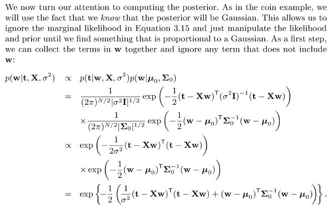
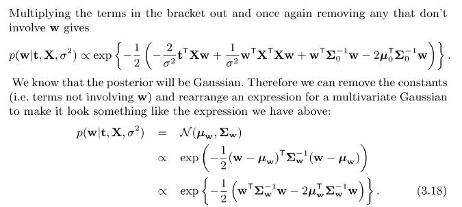
In Section 3.8 .4 we derived an expression for the Gaussian posterior for a linear model within the context of the Olympic \(100 \mathrm{~m}\) data. Substituting \(\boldsymbol{\mu}_{0}=\) \([0,0,
Redraw the graphical representation of the Olympic \(100 \mathrm{~m}\) model to reflect the fact that the prior over \(\mathbf{w}\) is actually conditioned on \(\boldsymbol{\mu}_{0}\) and
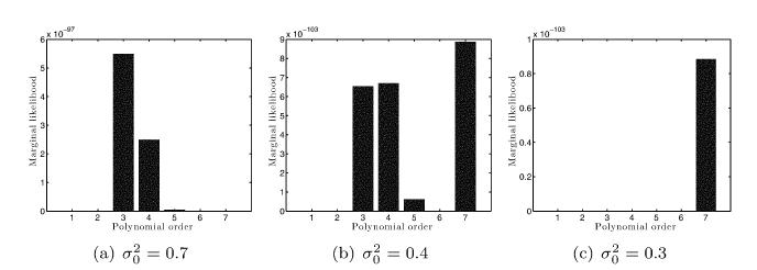
In Figure 3.25 we studied the effect of reducing \(\sigma_{0}^{2}\) on the marginal likelihood. Using MATLAB, investigate the effect of increasing \(\sigma_{0}^{2}\).Data from Figure 3.25 Marginal
When performing a Bayesian analysis on the Olympics data, we assumed that the prior was known. If a Gaussian prior is placed on \(\mathbf{w}\) and an inverse gamma prior on the variance
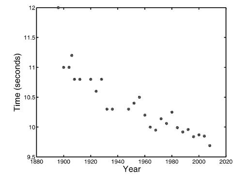
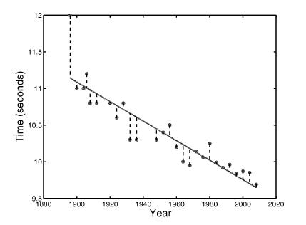
By examining Figure 1.1 estimate the kind of values we should expect for \(w_{0}\) and \(w_{1}\) (e.g. High? Low? Positive? Negative?).Data from Figure 1.1 Time (seconds) 10.5 101 12 11.5- 9.5 1880
Write a MATLAB script that can find \(w_{0}\) and \(w_{1}\) for an arbitrary dataset of \(x_{n}, t_{n}\) pairs.
Show that\[\mathbf{w}^{\top} \mathbf{X}^{\top} \mathbf{X} \mathbf{w}=w_{0}^{2}\left(\sum_{n=1}^{N} x_{n 1}^{2}\right)+2 w_{0} w_{1}\left(\sum_{n=1}^{N} x_{n 1} x_{n
Using \(\mathbf{w}\) and \(\mathbf{X}\) as defined in the previous exercise, show that \((\mathbf{X} \mathbf{w})^{\top}=\mathbf{w}^{\top} \mathbf{X}^{\top}\) by multiplying out both sides.
When multiplying a scalar by a vector (or matrix), we multiply each element of the vector (or matrix) by that scalar. For \(\mathbf{x}_{n}=\left[x_{n 1}, x_{n 2}\right]^{\top},
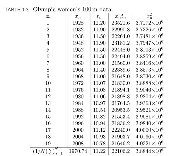
Using the data provided in Table 1.3 , find the linear model that minimises the squared loss.Data from Table 1.3 TABLE 1.3 Olympic women's 100 m data. n xn 1 1928 tn Intn 12.20 23521.6 3.7172106 x 2
Load the data stored in the file synthdata.mat. Fit a fourth-order polynomial function \(-f(x ; \mathbf{w})=w_{0}+w_{1} x+w_{2} x^{2}+w_{3} x^{3}+w_{4} x^{4}-\) to this data. What do you notice about
Derive the optimal least squares parameter value, \(\widehat{\mathbf{w}}\), for the total training loss\[\mathcal{L}=\sum_{n=1}^{N}\left(t_{n}-\mathbf{w}^{\top} \mathbf{x}_{n}\right)^{2}\]How does
The following expression is known as the weighted average loss:\[\mathcal{L}=\frac{1}{N} \sum_{n=1}^{N} \alpha_{n}\left(t_{n}-\mathbf{w}^{\top} \mathbf{x}_{n}\right)^{2}\]where the influence of each
Using \(K\)-fold cross-validation, find the value of \(\lambda\) that gives the best predictive performance on the Olympic men's \(100 \mathrm{~m}\) data for (a) a firstorder polynomial (i.e. the
Would the errors in the \(100 \mathrm{~m}\) linear regression (shown in Figure 2.1 ) be best modelled with a discrete or continuous random variable?Data from Figure 2.1 Time (seconds) 12 11.5 10.5 10
By using the fact that, when rolling a die, all outcomes are equally likely and by using the constraints given in Equations 2.1 and 2.2 , compute the probabilities of the dice landing with each of
\(Y\) is a random variable that can take any positive integer value. The likelihood of these outcomes is given by the Poisson pdf\[p(y)=\frac{\lambda^{y}}{y!} \exp \{-\lambda\}\]By using the fact
Assume that \(p(\mathbf{w})\) is the Gaussian pdf for a \(D\)-dimensional vector \(\mathbf{w}\) given in Equation 2.28 . By expanding the vector notation and rearranging, show that using
Using the same setup as Exercise 2.5 above, see what happens if we use a diagonal covariance matrix with different elements on the diagonal, i.e.\[\boldsymbol{\Sigma}=\left[\begin{array}{cccc}
Show that for a first-order polynomial, the diagonal elements of the Hessian matrix of second derivatives of the log-likelihood is equivalent to (they will differ by a multiplicative constant) the
Assume that a dataset of \(N\) values, \(x_{1}, \ldots, x_{N}\), was sampled from a Gaussian distribution. Assuming that the data are IID, find the maximum likelihood estimate of the Gaussian mean
Assume that a dataset of \(N\) binary values, \(x_{1}, \ldots, x_{N}\), was sampled from a Bernoulli. Compute the maximum likelihood estimate for the Bernoulli parameter.
Obtain the maximum likelihood estimates of the mean vector and covariance matrix of a multivariate Gaussian density given \(N\) observations \(\mathbf{x}_{1}, \ldots, \mathbf{x}_{N}\).
Show that the maximum likelihood estimate of the noise variance in our linear model,\[\widehat{\sigma^{2}}=\frac{1}{N}\left(\mathbf{t}^{\top} \mathbf{t}-\mathbf{t}^{\top} \mathbf{X}

Step by Step Answers

Services

Sitemap
Fun
Definitions
Become Tutor
Used Textbooks
Study Help Categories
Recent Questions
Expert Questions

Company Info

Security
Copyrights
Privacy Policy
Terms & Conditions
SolutionInn Fee
Scholarship

Get In Touch

About Us
Contact Us
Career
Jobs
FAQ
Campus Ambassador

Secure Payment

Download Our App

© 2025 SolutionInn. All Rights Reserved