Nuclear plants Here are data on 32 light water nuclear power plants. The variables are:

. Cost: In $100,000, adjusted to 1976 base.

. Date: Date that construction permit was issued in years after 1900. Thus, 68.58 is roughly halfway through 1968.

. Mwatts: Power plant net capacity in megawatts.

. We are interested in the Cost of the plants as a function of Date and Mwatts.

1. Examine the relationships between Cost and Mwatts and between Cost and Date. Make appropriate displays and interpret them with a sentence or two.

2. Find the regression of Cost on Mwatts. Write a sentence that explains the relationship as described by the regression.

3. Make a scatterplot of residuals vs. predicted values and discuss what it shows. Make a Normal probability plot or histogram of the residuals. Discuss the four assumptions needed for regression analysis and indicate whether you think they are satisfied here. Give your reasons.

4. State the standard null hypothesis for the slope coefficient and complete the t-test at the 5% level. State your conclusion.

5. Estimate the cost of a 1000-mwatt plant. Show your work.

6. Compute the residuals for this regression. Discuss the meaning of the R-squared in this regression. Plot the residuals against Date. Does it appear that Date can account for some of the remaining variability?

7. Compute the multiple regression of Cost on both Mwatts and Date. Compare the coefficient in this regression with those you have found for each of these predictors.

8. Would you expect Mwatts and Date to be correlated? Why or why not? Examine the relationship between Mwatts and Date. Make a scatterplot and find the correlation coefficient, for example. It’s only because of the extraordinary nature of this relationship that the relationships you saw at earlier steps were this simple.

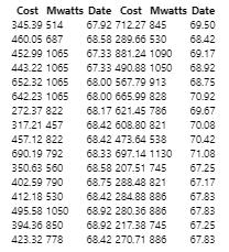
Cost Mwatts Date Cost Mwatts Date 67.92 712.27 845 69.50 68.58 289.66 530 68.42 67.33 881.24 1090 69.17 67.33 490.88 1050 68.92 68.00 567.79 913 68.75 345.39 514 460.05 687 452.99 1065 443.22 1065 652.32 1065 642.23 1065 272.37 822 317.21 457 457.12 822 690.19 792 350.63 560 402.59 790 412.18 530 495.58 1050 394.36 850 423.32 778 68.00 665.99 828 68.17 621.45 786 68.42 608 80 821 68.42 473.64 538 68.33 697.14 1130 68.58 207.51 745 68.75 288.48 821 68.42 284.88 886 68.92 280.36 886 68.92 217.38 745 68.42 270.71 886 70.92 69.67 70.08 70.42 71.08 67.25 67.17 67.83 67.83 67.25 67.83