We wish to estimate the hedonic regression model

The variables are PRICE (\\($1000),\) SQFT (100s), CLOSE = 1 if located near a major university, 0 otherwise, AGE (years), FIREPLACE, POOL, TWOSTORY \(=1\) if present, 0 otherwise.

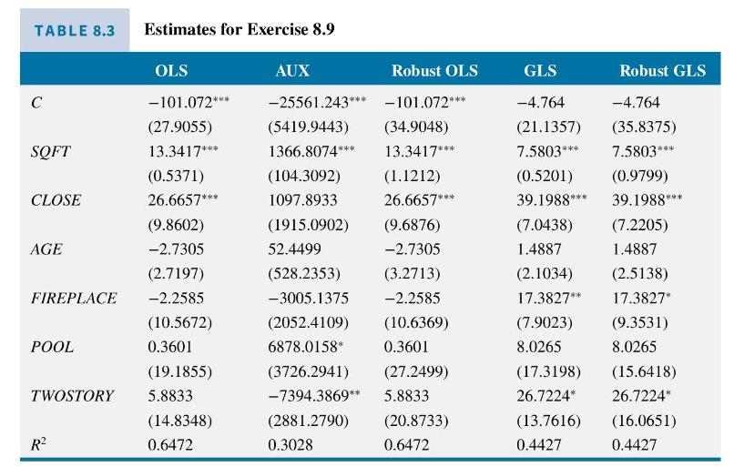
a. Using Table 8.3, comment on the sign, significance, and interpretation of the OLS coefficient estimate for the variable CLOSE.

b. Answer each of the following True or False. In a regression model with heteroskedasticity, (i) the OLS estimator is biased; (ii) the OLS estimator is inconsistent; (iii) the OLS estimator does not have an approximate normal distribution in large samples; (iv) the usual OLS standard error is too small; (v) the usual OLS estimator standard error is incorrect; (vi) the usual \(R^{2}\) is no longer meaningful; (vii) the usual overall \(F\)-test is reliable in large samples.

c. Following the OLS regression, the residuals are saved as EHAT. In the regression labeled AUX in Table 8.3, the dependent variable is \(E H A T^{2}\). Test for the presence of heteroskedasticity, using the \(5 \%\) level of significance. State the test statistic, the test critical value, and your conclusion.

d. The model is reestimated by OLS using White heteroskedasticity-consistent standard errors. In what way are these standard errors robust? Are they valid when there is homoskedasticity, heteroskedasticity, in small samples and large? Which of the statistically significant coefficients has wider confidence intervals using the robust standard errors? Do any coefficients switch from being significant at \(5 \%\) to not significant at \(5 \%\), or vice versa?

e. Our researcher estimates the equation after dividing each variable, and the constant term, by \(S Q F T\) to obtain the GLS estimates. What assumption has been made about the form of heteroskedasticity in this estimation? Are the GLS estimates, shown in Table 8.3, noticeably different from the OLS estimates? Do any coefficients switch from being significant at \(5 \%\) to not significant at \(5 \%\), or vice versa?

f. The residuals from the transformed regression in part (e) are called ESTAR. The researcher regresses \(E S T A R^{2}\) on all the transformed variables and includes an intercept. The \(R^{2}=0.0237\). Has the researcher eliminated heteroskedasticity?

g. The researcher estimates the model in (e) again but uses robust standard errors. These are reported in Table 8.3 as "Robust GLS." Do you consider this a prudent thing to do? Explain your reasoning.

Transcribed Image Text:

= PRICE, B+SQFT; +3CLOSE, + AGE; + FIREPLACE, +POOL +B,TWOSTORY; + e;