Un conventional monetary policy: financial policy and quantitative easing We have written the IS-LM model in terms:
Question:
Un conventional monetary policy: financial policy and quantitative easing We have written the IS-LM model in terms:
\[
\begin{align*}
\text { IS relation: } & Y=C(Y-T)+I(Y, r+x)+G \tag{6.5}\\
L M \text { relation: } & r=\bar{r} \tag{6.6}
\end{align*}
\]
Interpret the interest rate as the federal funds rate adjusted for expected inflation, the real policy interest rate of the Federal Reserve. Assume that the rate at which firms can borrow is much higher than the federal funds rate, equivalently that the premium, \(x\), in the IS equation is high.
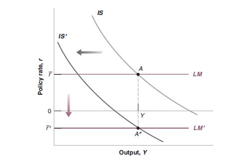
a. Suppose that the government takes action to improve the solvency of the financial system. If the government's action is successful and banks become more willing to lend-both to one another and to nonfinancial firms - what is likely to happen to the premium? What will happen to the IS-LM diagram based on Figure 6-6? Can we consider financial policy as a kind of macroeconomic policy?
b. Faced with a zero nominal interest rate, suppose the Fed decides to purchase securities directly to facilitate the flow of credit in the financial markets. This policy is called quantitative easing. If quantitative easing is successful, so that it becomes easier for financial and nonfinancial firms to obtain credit, what is likely to happen to the premium? What effect will this have on the IS-LM diagram? If quantitative easing has some effect, is it true that the Fed has no policy options to stimulate the economy when the federal funds rate is zero?
c. We will see later in the course that one argument for quantitative easing is that it increases expected inflation. Suppose quantitative easing does increase expected inflation. How does that affect the LM curve in Figure 6-6?
Figure 6-6

Step by Step Answer:


