Piston Corporation (part A). Reginald Jackson was employed as cos accountant by the piston corporation. A medium size auto parts company located in the out stroke of Detroit Kelly Jones, the controller for piston, decide that she needed an assistant. Jackson was selected to fill that position. As part of his training program, Jackson was sent to night school to study quantitative applications in cost accounting.

Because the piston corporation?s products were replacement parts, its salsas were, fortunately, not as volatile as the new car market?s. Piston had experienced a rather stable growth in sales in recent years and had been reared to increase its capacity regularly. It appeared to be time for another expansion but in an uncertain stock market prevailing and uncertainty concerning interest rates. Jones was worried about obtaining funds at a reasonable cost. On the other hand piston?s production manager had been complaining more than usual about various personnel Material handling and scheduling bottlenecks that arose from the high level of output demanded of his present facilities.

The executive officers had been asked by piston?s directors to formulate a proposal for expansion and price adjustments. Jones asked Jackson what he could determine statistically about the effect of inflation and the level of production on unit cost.

By looking at old budgets Jackson was able to obtain quarterly data on manufacturing costs per unit. Production level (a percentage of the total capacity).and the index of direct material and direct labor costs for a five Year period (These data are in a tile PISTONS on the CD.He immediately went to the computer and ran regression of unit cost on production volume (PROD) and The cost index (INDEX), He began to wonder about the validity of modeling unit costs as a linear function of production level and the cost index.

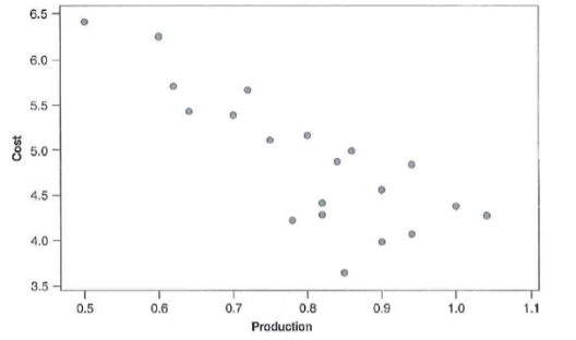
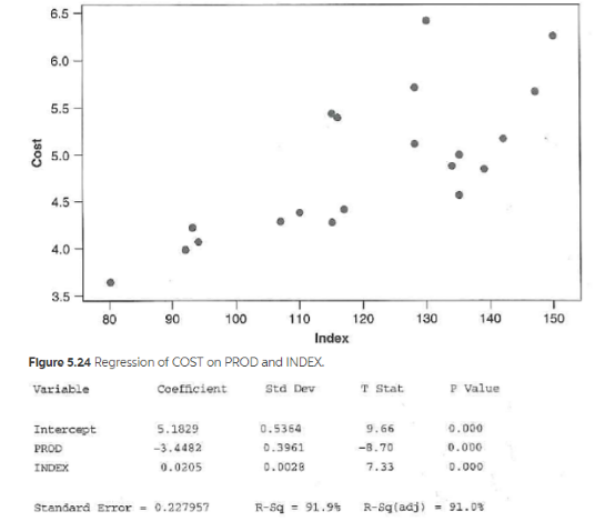
The scatter plots of the dependent variable (COST) versus each explanatory variable arc shown in Figures 5.22 and 523.The regression results are in Figure 5.24 . After spending several day, trying to improve his model. Jackson had several new solutions but was still unsure which one was best. That night after his quantitative accounting he asked his professor for advice. The professor suggested Jackson first derive a theoretically plausible solution and then see it the data satisfied this relationship, Jackson knew that basic relationship with which he was dealing was:

Total cost = variable cost per unit x volume + fixed cost

He also theorized that variable cost per unit was composed of a constant multiple of the Index of direct materials and labor(x ₂ ) and that fixed cost was simply the current capacity of the company times some constant.

Jackson realized that the basic equation could rewritten as:

total cost = ? ₁ capacity volume + ? ₂ x ₂ volume

Then it dawned on him that he actually wanted cost per unit. The preceding equation could be divided by volume to get

Total cost = ? ₁ capacity + ? ₂ x ₂

Capacity/volume. However, is simply the reciprocal of production level. so the new equation becomes

Where y is total cost/volume (or cost per unit), is production level and X2 Is cost index. Allowing for random error and allowing the equation to have an intercept term produces:

Try Jackson's new model. How does this model compare with the original regression? In answering this question. Use the R2 values, The standard error of the regression and any other information you feel might be useful in the comparisons, Which model do you prefer?

Figure 5.22 scatterplot of COST versus PROD

Scatterplot of cost versus PROD

Figure 5.23 scatterplot of cost versus INDEX

Scatter plot of cost versus INDEX

y = P( ) + + Bx2 _' = Bo + B ( =) = + Bx + e Cost 6.5 6.0 5.5 5.0 4.5 4.0 3.5 I T I I T 0.5 0.6 0.7 0.8 Production 0.9 1.0 1.1 Cost 6.5 6.0 5.5 5.0 T T 4.0 3.5 4.5- T T Intercept PROD INDEX 80 90 5.1829 -3.4482 0.0205 100 Figure 5.24 Regression of COST on PROD and INDEX. Variable Coefficient Std Dev Standard Error 0.227957 110 Index 0.5364 0.3961 0.0028 R-Sq 91.9% 120 T Stat 9.66 -8.70 7.33 130 140 P Value 0.000 0.000 0.000 R-Sq(adj) Analysis of Variance Source DF Regression 2 17 19 Error Total Sum of Squares 10.0586 0.8834 10.9420 Mean Square 5.0293 0.0520 F Stat 96.78 P Value 0.000