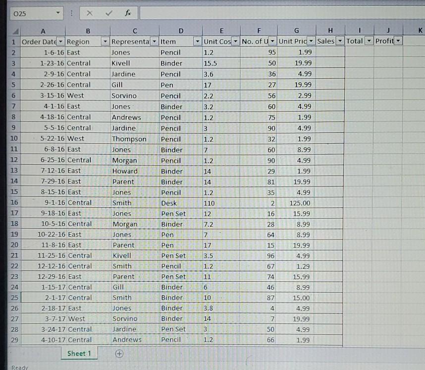
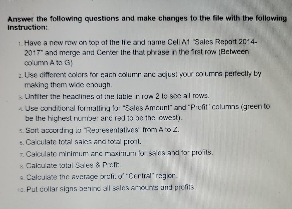
025 X fa K Total Profit 15.5 A B 1 Order Date Region 2 1-6-16 East 3 1-23-16 Central 4 2-9-16 Central 5 2-26-16 Central 3-15-16 West 7 4-1-16 East 8 4-18-16 Central 9 5-5-16 Central 10 5-22-16 West 111 6-8-16 East 12 6-25-16 Central 13 7-12-16 East 14 7-29-16 East D Representatem Jones Pencil Kivell Binder Jardine Pencil Gill Pen Sorvino Pencil Jones Binder Andrews Pencil Jardine Pencil Thompson Pencil Jones Binder Morgan Pencil Howard Binder Parent Binder Jones Pencil Smith Desk Jones Pen Set Morgan Binder Jones Pen Parent Pen Kivell Pen Set Smith Pencil Parent Pen Set Gill Binder Smith Binder Jones Binder Sorvino Binder Jardine Pen Set Andrews Pencil E F G Unit CosNo. of Unit Pric Sales 1.2 95 1.99 50 19.99 3.6 36 4.99 17 27 19.99 2.2 56 2.99 3.2 60 4.99 1.2 75 1.99 3 90 4.99 1.2 32 1.99 7 60 8.99 1.2 90 4.99 14 29 1.99 14 81 19.99 1.2 35 4.99 110 2 125.00 12 16 15.99 8.99 7 64 8.99 17 15 19.99 3.5 96 4.99 1.2 67 1.29 11 74 15.99 6 46 8.99 10 87 15.00 3.8 4 4.99 14 7 19.99 3 50 4.99 1.2 66 1.99 15 16 17 18 7.2 28 19 20 21 22 8-15-16 East 9-1-16 Central 9-18-16 East 10-5-16 Central 10-22-16 East 11-8-16 East 11-25-16 Central 12-12-16 Central 12-29-16 East 1-15-17 Central 2-1-17 Central 2-18-17 East 3 17 West 3-24-17 Central 4-10-17 Central 23 NNNNNN Sheet 1 Ready Answer the following questions and make changes to the file with the following instruction: 1. Have a new row on top of the file and name Cell A1 "Sales Report 2014- 2017" and merge and Center the that phrase in the first row (Between column A to G) 2. Use different colors for each column and adjust your columns perfectly by making them wide enough. 3. Unfilter the headlines of the table in row 2 to see all rows. 4. Use conditional formatting for "Sales Amount" and "Profit" columns (green to be the highest number and red to be the lowest). 5. Sort according to "Representatives" from A to Z. 6. Calculate total sales and total profit. 7. Calculate minimum and maximum for sales and for profits. 8. Calculate total Sales & Profit. 9. Calculate the average profit of "Central" region. 10. Put dollar signs behind all sales amounts and profits. 025 X fa K Total Profit 15.5 A B 1 Order Date Region 2 1-6-16 East 3 1-23-16 Central 4 2-9-16 Central 5 2-26-16 Central 3-15-16 West 7 4-1-16 East 8 4-18-16 Central 9 5-5-16 Central 10 5-22-16 West 111 6-8-16 East 12 6-25-16 Central 13 7-12-16 East 14 7-29-16 East D Representatem Jones Pencil Kivell Binder Jardine Pencil Gill Pen Sorvino Pencil Jones Binder Andrews Pencil Jardine Pencil Thompson Pencil Jones Binder Morgan Pencil Howard Binder Parent Binder Jones Pencil Smith Desk Jones Pen Set Morgan Binder Jones Pen Parent Pen Kivell Pen Set Smith Pencil Parent Pen Set Gill Binder Smith Binder Jones Binder Sorvino Binder Jardine Pen Set Andrews Pencil E F G Unit CosNo. of Unit Pric Sales 1.2 95 1.99 50 19.99 3.6 36 4.99 17 27 19.99 2.2 56 2.99 3.2 60 4.99 1.2 75 1.99 3 90 4.99 1.2 32 1.99 7 60 8.99 1.2 90 4.99 14 29 1.99 14 81 19.99 1.2 35 4.99 110 2 125.00 12 16 15.99 8.99 7 64 8.99 17 15 19.99 3.5 96 4.99 1.2 67 1.29 11 74 15.99 6 46 8.99 10 87 15.00 3.8 4 4.99 14 7 19.99 3 50 4.99 1.2 66 1.99 15 16 17 18 7.2 28 19 20 21 22 8-15-16 East 9-1-16 Central 9-18-16 East 10-5-16 Central 10-22-16 East 11-8-16 East 11-25-16 Central 12-12-16 Central 12-29-16 East 1-15-17 Central 2-1-17 Central 2-18-17 East 3 17 West 3-24-17 Central 4-10-17 Central 23 NNNNNN Sheet 1 Ready Answer the following questions and make changes to the file with the following instruction: 1. Have a new row on top of the file and name Cell A1 "Sales Report 2014- 2017" and merge and Center the that phrase in the first row (Between column A to G) 2. Use different colors for each column and adjust your columns perfectly by making them wide enough. 3. Unfilter the headlines of the table in row 2 to see all rows. 4. Use conditional formatting for "Sales Amount" and "Profit" columns (green to be the highest number and red to be the lowest). 5. Sort according to "Representatives" from A to Z. 6. Calculate total sales and total profit. 7. Calculate minimum and maximum for sales and for profits. 8. Calculate total Sales & Profit. 9. Calculate the average profit of "Central" region. 10. Put dollar signs behind all sales amounts and profits