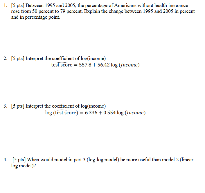
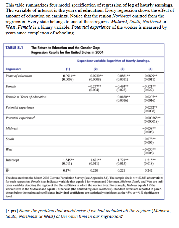
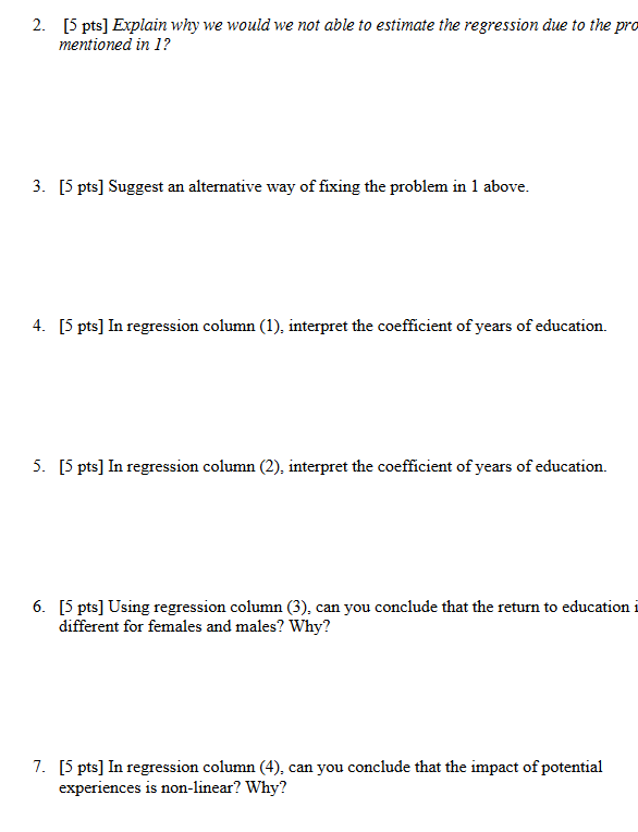
1. [5 pts] Between 1995 and 2005, the percentage of Americans without health insurance rose from 50 percent to 79 percent. Explain the change between 1995 and 2005 in percent and in percentage point. 2. [5 pts] Interpret the coefficient of log(income) test score = 557.8 + 56.42 log (Income) 3. [5 pts ] Interpret the coefficient of log(income) log (test score) = 6.336 + 0.554 log (Income) 4. [5 pts] When would model in part 3 (log-log model) be more useful than model 2 (linear- log model)?This table summarizes four model specification of regression of log of hourly earnings. The variable of interest is the years of education. Every regression shows the effect of amount of education on earnings. Notice that the region Northeast omitted from the regression. Every state belongs to one of these regions: Midwest, South, Northeast or West. Female is a binary variable. Potential experience of the worker is measured by years since completion of schooling. TABLE 8.1 The Return to Education and the Gender Gap: Regression Results for the United States in 2004 Dependent variable: logarithm of Hourly Earnings. Regresson (1) (2) (3) (4) Years of education 0.0914+ 0.0930* 0.0861 (0.0008) 0.0899#* (0.0008) (0.0011) (0.0011) Female -0.237 -0.484** -0.521** (0.004) (0.023) (0.022) Female X Years of education 0.0180* 0.0207** (0.0016) (0.0016) Potential experience 0.0232** (0.0008) Potential experience -0.000368* (0.000018) Midwest -0.058** (0.006) South -0.078* (0.006) West -0.030** (0.006) Intercept 1.545* 1.621.* (0.011) 1.721*. 1.215.* (0.011) (0.015) (0.018) R 0.174 0.220 0.221 0.242 The data are from the March 2005 Current Population Survey (see Appendix 3.1). The sample size is a = 57,863 observations for each regression. Female is an indicator variable that equals 1 for women and O for men. Midwest, South, and West are indi- cator variables denoting the region of the United States in which the worker lives For example, Midwest equals 1 if the worker lives in the Midwest and equals 0 otherwise (the omitted region is Northeast). Standard errors are reported in paren- theses below the estimated coefficients Individual coefficients are statistically significant at the *5% or *#1% significance level. [5 pts] Name the problem that would arise if we had included all the regions (Midwest, South, Northeast or West) at the same time in our regression?2. [5 pts] Explain why we would we not able to estimate the regression due to the pro mentioned in 1? 3. [5 pts] Suggest an alternative way of fixing the problem in 1 above. 4. [5 pts] In regression column (1), interpret the coefficient of years of education. 5. [5 pts] In regression column (2), interpret the coefficient of years of education. 6. [5 pts] Using regression column (3). can you conclude that the return to education different for females and males? Why? 7. [5 pts] In regression column (4), can you conclude that the impact of potential experiences is non-linear? Why?1. You work for a retail store and are interested in the relationship between rainy days and sales. Sales is monthly sales in thousands of dollars. Rain is the number of rainy days in a month. reg sales rainy days Source 55 df MS Number of obs = 120 F( 1, 118) = 3.53 Model 1178 . 75035 1 1178. 75035 Prob > F 0. 0628 Residual 39434. 1325 118 334. 187564 R-squared Adj R-squared = Total 40612 . 8829 119 341. 28473 Root MSE 18. 281 sales Coef. 5td. Err. t P>ItI [954 Conf. Interval] rainy_days 8978109 -1. 88 0. 063 -3. 464077 . 0917428 cons 27.27458 6. 668928 4. 09 0. 000 14. 06829 40 . 48088 a) [5 pts] From the output shown above calculate the R 2 value. Show your work. b) [5 pts] Based on the any method of your liking from the table above can you conclude if rainy days' impact sales? (use o=0.05, and t-critical value = 2)In a similar spirit with the RAND health insurance experiment, the state of Oregon randomly selected winners and losers of lotteries, and give free health insurance to lottery winners. This generates a randomized control trial, with the lottery winners being the treatment group and losers being the control group. The following table shows outcomes from this research for the sample of whole Oregon and the sample of Portland area only. For both samples, the mean of control group and the difference between treatment and control are listed in different columns. Standard errors reported in parentheses. Treatment effect picks up the difference between control mean and treatment mean. Oregon Portland area Control Treatment Control Treatment mean effect mean effect Outcome (1) (2) (3) (4) A. Administrative data Ever on Medicaid 141 .256 151 .247 (.004) (.006) Any hospital admissions .067 .005 (.002) Any emergency department 345 .017 visit (.006) Number of emergency 1.02 .101 department visits (.029) Sample size 74,922 24,646 B. Survey data Outpatient visits (in the 1.91 .314 past 6 months (.054) Any prescriptions? 637 .025 (.008) Sample size 23,7411. [10 pts] Compare the treatment effect estimates (Ever on Medicaid, any emergency department visit) with the control means for the Portland area. Explain the estimate and if possible say something about the size of the effect. 2. [10 pts] Perform statistical inference on the difference between the treatment (Ever on Medicaid, Any emergency department) and control to see if each of these 2 estimates are statistically significant at 0=0.05. (Hint: use rule of thumb: compare t-stat with t- critical value of 2).Part V (10 points) 1. [5 pts] Suppose you're interested in estimating the effect of family income (In thousands of dollars) on number of ideal kids a couple wants to have. Your original model is given as follows: Number of ideal Kids = Bo + , family income + u (a) How would you change the model if you think that the effect of family income on number of ideal kids can be different for immigrant and non-immigrant couples? (b) In the modified model in (a), how would you test whether there is a differential effect of family income on the ideal number of kids that a couple wants to have depending on immigrant status? State the null hypothesis and alternative hypothesis. Part VI [20 pts] Answer any four of the 5 questions. 1. [5 pts] What does it mean for a study to externally valid? Give an example. 2. [5 pts] How is R-square different from adjusted R-square?3. [5 pts] Name 5 potential sources of bias in a multiple regression. 4. [5 pts] Explain 'Izairh},r the naive comparison is not misleading in the case of a randomized control trial? 5. [5 pts] How would you check before the experiment that the randomization has been done well?r