

Question: 1. Create the following table in Sheet1, starting from the cell A1 A B C D E F G H 1 Easy Mobile 2 Code
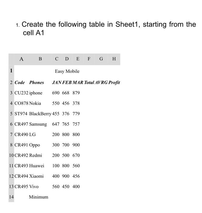
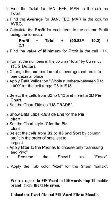
1. Create the following table in Sheet1, starting from the cell A1 A B C D E F G H 1 Easy Mobile 2 Code Phones JAN FEB MAR Total AVRG Profit 3 CU232 iphone 690 668 879 4 C0878 Nokia 550 456 378 5 ST974 BlackBerry 455 376 779 6 CR497 Samsung 647 765 757 7 CR490 LG 200 800 800 8 CR491 Oppo 300 700 900 10 CR492 Redmi 200 500 670 11 CR493 Huawei 100 800 560 12 CR494 Xiaomi 400 900 456 13 CR495 Vivo 560 450 400 14 Minimum 2. Find the Total for JAN, FEB, MAR in the column Total. 3. Find the Average for JAN, FEB, MAR in the column AVRG. 4. Calculate the Profit for each item, in the column Profit using the formula. Profit - Total (99.88* 10.2) 1 2.3 5. Find the value of Minimum for Profit in the cell H14. + 6. Format the numbers in the column "Total" by Currency $(US Dollar). 7. Change the number format of average and profit to one decimal place 8. Apply Data Validation "Whole numbers-between 0 to 1000" for the cell range C3 to E13. 1. Select the cells from B2 to C13 and insert a 3D Pie Chart 2 Set the Chart Title as "US TRADE". 3. Show Data Label-Outside End for the Pie chart 4. Set the Chart style -7 for the Pie chart 5. Select the cells from B2 to H6 and Sort by column profit in the order of smallest to largest 6. Apply filter to the Phones to choose only "Samsung and Vivo" Rename the Sheet1 as "Emax". 8. Apply the Tab color "Red" for the Sheet "Emax". 7. Write a report in MS Word in 100 words top 10 mobile brand" from the table given. Upload the Excel file and MS Word File to Moodle. 1. Create the following table in Sheet1, starting from the cell A1 A B C D E F G H 1 Easy Mobile 2 Code Phones JAN FEB MAR Total AVRG Profit 3 CU232 iphone 690 668 879 4 C0878 Nokia 550 456 378 5 ST974 BlackBerry 455 376 779 6 CR497 Samsung 647 765 757 7 CR490 LG 200 800 800 8 CR491 Oppo 300 700 900 10 CR492 Redmi 200 500 670 11 CR493 Huawei 100 800 560 12 CR494 Xiaomi 400 900 456 13 CR495 Vivo 560 450 400 14 Minimum 2. Find the Total for JAN, FEB, MAR in the column Total. 3. Find the Average for JAN, FEB, MAR in the column AVRG. 4. Calculate the Profit for each item, in the column Profit using the formula. Profit - Total (99.88* 10.2) 1 2.3 5. Find the value of Minimum for Profit in the cell H14. + 6. Format the numbers in the column "Total" by Currency $(US Dollar). 7. Change the number format of average and profit to one decimal place 8. Apply Data Validation "Whole numbers-between 0 to 1000" for the cell range C3 to E13. 1. Select the cells from B2 to C13 and insert a 3D Pie Chart 2 Set the Chart Title as "US TRADE". 3. Show Data Label-Outside End for the Pie chart 4. Set the Chart style -7 for the Pie chart 5. Select the cells from B2 to H6 and Sort by column profit in the order of smallest to largest 6. Apply filter to the Phones to choose only "Samsung and Vivo" Rename the Sheet1 as "Emax". 8. Apply the Tab color "Red" for the Sheet "Emax". 7. Write a report in MS Word in 100 words top 10 mobile brand" from the table given. Upload the Excel file and MS Word File to Moodle
Step by Step Solution
There are 3 Steps involved in it

Get step-by-step solutions from verified subject matter experts