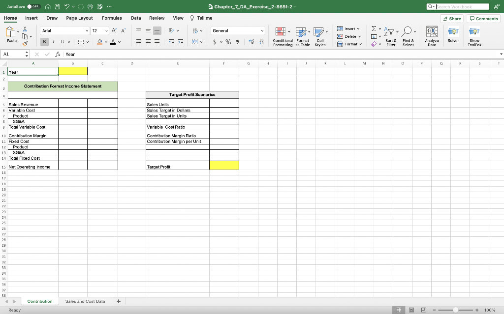
1. Enter the year 2019 into cell B1 on the Contribution worksheet.

2. Enter a CONCATENATE function into the merged cell beginning with cell A4 on the Contribution worksheet. The function should combine the words Fiscal Year: and the year that is entered into cell B1. Note that there are two spaces that should be added after the colon following the words Fiscal Year.

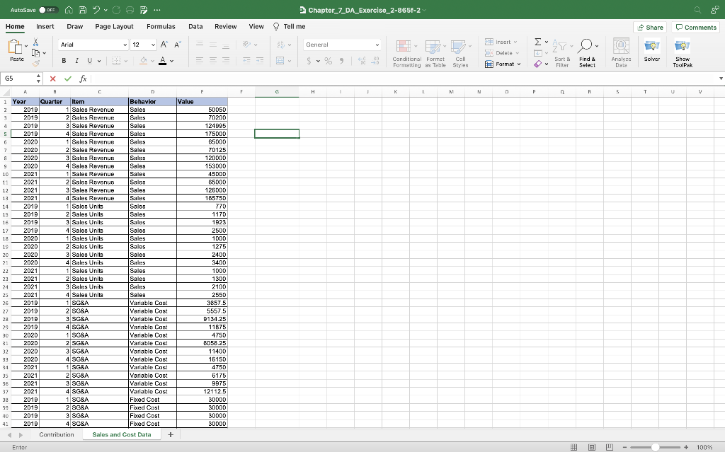
3. Enter a SUMIFS function into cell C5 on the Contribution worksheet that sums the Sales Revenue on the Sales and Cost Data worksheet based on the year that is entered into cell B1 on the Contribution worksheet. The data to be summed is in column E on the Sales and Cost Data worksheet. The function should find a match in the Year column on the Sales and Cost Data worksheet to the year entered in cell B. The function should also find a match to the item in cell A5 (Sales Revenue) in column C on the Sales and Cost Data worksheet. Add cell capacity to include row 100 on the Sales and Cost Data worksheet.

4. Enter a SUMIFS function into cell B7 on the Contribution worksheet that sums the variable product costs on the Sales and Cost Data worksheet. The setup of this function is identical to the SUMIFS function in step 3 with the following changes: This function should find a match to the item in cell A7 (Product) in column C on the Sales and Cost Data worksheet. This function should also find a match to the item in cell A6 (Variable Cost) in column D on the Sales and Cost Data worksheet. Add cell capacity to include row 100 on the Sales and Cost Data worksheet.

5. Enter a SUMIFS function into cell B8 on the Contribution worksheet that sums the variable SG&A costs on the Sales and Cost Data worksheet. The setup of this function is identical to the SUMIFS function in step 4 except this function should find a match to the item in cell A8 (SG&A) in column C on the Sales and Cost Data worksheet. Add cell capacity to include row 100 on the Sales and Cost Data worksheet.

6. Enter a formula in cell C9 on the Contribution worksheet that sums the two variable costs in cells B7 and B8.

7. Enter a formula in cell C10 that calculates the Contribution Margin. The formula should subtract the total variable costs in cell C9 from the sales revenue in cell C5 (C5-C9).

8. Enter a SUMIFS function into cell B12 on the Contribution worksheet that sums the fixed product costs on the Sales and Cost Data worksheet. The setup of this function is identical to the SUMIFS function in step 4 with the following changes: This function should find a match to the item in cell A12 (Product) in column C on the Sales and Cost Data worksheet. This function should also find a match to the item in cell A11 (Fixed Cost) in column D on the Sales and Cost Data worksheet. Add cell capacity to include row 100 on the Sales and Cost Data worksheet.

9. Enter a SUMIFS function into cell B13 on the Contribution worksheet that sums the fixed SG&A costs on the Sales and Cost Data worksheet. The setup of this function is identical to the SUMIFS function in step 8 except this function should find a match to the item in cell A13 (SG&A) in column C on the Sales and Cost Data worksheet. Add cell capacity to include row 100 on the Sales and Cost Data worksheet.

10. Enter a formula in cell C14 on the Contribution worksheet that sums the two fixed costs in cells B12 and B13.

11. Enter a formula in cell C15 that calculates the Net Operating Income. The formula should subtract the total fixed costs in cell C14 from the contribution margin in cell C10 (C10-C14).

12. Enter a SUMIFS function into cell F5 on the Contribution worksheet that sums the Sales Units on the Sales and Cost Data worksheet. The setup of this function is identical to the SUMIFS function in step 3 that was used to calculate the Sales Revenue. However, this function should find a match to the item in cell E5 (Sales Units) in column C on the Sales and Cost Data worksheet. Add cell capacity to include row 100 on the Sales and Cost Data worksheet.

13. Enter the value 60000 into cell F15 on the Contribution worksheet. The first scenario will calculate sales targets in order for the company to achieve a net operating income of $60,000.

14. Enter a formula into cell F11 that calculates the contribution margin per unit. The formula should divide the contribution margin in cell C10 by the Sales Units in cell F5.

15. Enter a formula into cell F9 that calculates the variable cost ratio. This formula should divide the total variable cost in cell C9 by the sales revenue in cell C5.

16. Enter a formula into cell F10 that calculates the contribution margin ratio. This formula should subtract from the number 1 the variable cost ratio in cell F9. The contribution margin ratio and the variable cost ratios are percentages of the sales revenue. When added together, these ratios must equal 1 or 100%.

17. Enter a formula in cell F7 that calculates the Sales Target in Units which is needed to achieve the net operating income of $60,000. The formula should first add the target profit in cell F15 to the total fixed costs in cell C14. This result should be divided by the contribution margin per unit in cell F11.

18. Enter a formula in cell F6 that calculates the Sales Target in Dollars which is needed to achieve the net operating income of $60,000. The formula should first add the target profit in cell F15 to the total fixed costs in cell C14. This result should be divided by the contribution margin ratio in cell F10. The results show that based on the contribution format income statement for 2019, in order for the company to achieve $60,000 in net operating income, sales revenue must be $436,721. Sales in units must be 6,612. These results will change from year to year as the cost and sales data change.

19. Change the year in cell B1 to 2020. Notice the company is showing a loss of (12,106) with sales revenue at $408,125.

20. Change the value in cell F15 to 0. Notice the Sales Target in Dollars $437,554. This is known as the break even point. In order for the company to break-even with a net operating income of 0, the sales revenue must be $437,554. Note the sales revenue for 2020 is lower than this value, which is why the net operating income is less than 0.

21. Save and close your workbook.

D Chapter_7_DA_Exercise_2-865f-2 Qu kearch Workbook Tell me \& 4 Share Comments General $%,6,4% -46 Show show Toolpak \begin{tabular}{|l|l|} \hline \multicolumn{2}{|c|}{ Target Profit Scenarios } \\ \hline Sales Units & \\ \hline Sales Targetin Dollars & \\ \hline Saleg Targetin Units & \\ \hline Variable CostRatio & \\ \hline Centritastion Margin Ratio & \\ \hline Contribution Margin per Unit & \\ \hline & \\ \hline TargetProfit & \\ \hline \end{tabular} D Chapter_7_DA_Exercise_2-865f-2 Qu kearch Workbook Tell me \& 4 Share Comments General $%,6,4% -46 Show show Toolpak \begin{tabular}{|l|l|} \hline \multicolumn{2}{|c|}{ Target Profit Scenarios } \\ \hline Sales Units & \\ \hline Sales Targetin Dollars & \\ \hline Saleg Targetin Units & \\ \hline Variable CostRatio & \\ \hline Centritastion Margin Ratio & \\ \hline Contribution Margin per Unit & \\ \hline & \\ \hline TargetProfit & \\ \hline \end{tabular}