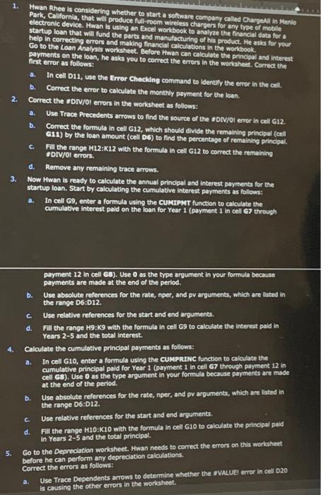
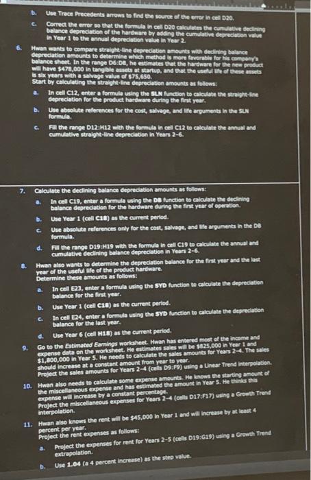
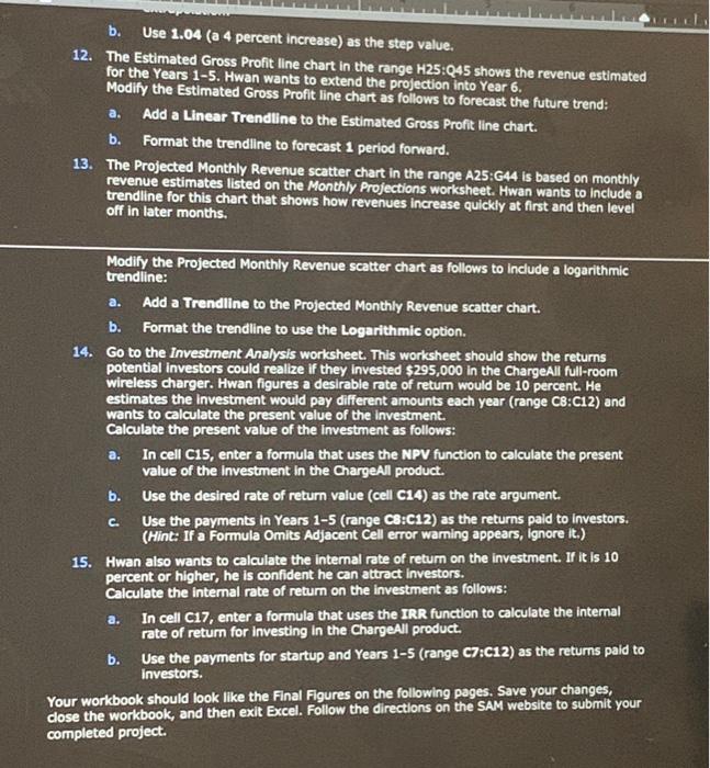
1. Hwan Rhee is considering whether to start a software company called Chargeali in Menlo Park, Californla, that will produce full-room wireless chargers for amy type of moblle electronic device. Hwan is using an Excel worlbook to analyze the financial data for a startup loan that will fund the parts and manufacturing of his product. He asks for your help in correcting errors and making financial calculations in the workbook. Go to the Loan Analysis workheet Belore Hwan can calculate the princlpel and interest payments on the loan, he asks you to correct the errors in the workshect. Correct the first error as follows: a. In cell D11, use the Error checklng command to identify the error in the cell. b. Correct the error to calculate the monthly payment for the loen. 2. Correct the oIV/OI errors in the worksheet as follows: a. Use Trace Precedents arrows to find the source of the oDVVol error in cell G12. b. Correct the formula in cell G12, which should divide the remaining principal (cell G12) by the loan amount (cell b6) to find the percentage of remaining principal. c. Fill the range H12:K12 with the formula in cell G12 to correct the remaining BDV/0i errors. d. Remove any remaining trace arrows. 3. Now Hwan is ready to caiculate the annual principal and interest payments for the startup loan. Start by calculating the cumulative interest payments as follows: a. In cell 69 , enter a formula using the CUMPMT function to calculate the cumulatlve interest pald on the loan for Year 1 (payment 1 in cell G7 through peyment 12 in cell G8), Use 0 as the type argument in your formula because payments are made at the end of the period. b. Use absolute references for the rate, nper, and pv arguments, which are listed in the range D6:D12. c. Use relative references for the start and end arguments. d. Fill the range H9:K9 with the formula in cell 69 to calculate the interest paid in Years 2-5 and the total interest. 4. Calculate the cumulative principal payments as follows: a. In cell G10, enter a formula using the cUMPRINC function to caloulate the cumulative principal pald for Year 1 (payment 1 in cell G7 through payment 12 in cell G8). Use 0 as the type argument in your formula because payments are made at the end of the period. b. Use absolute references for the rate, nper, and pv arguments, which are listed in the range D6:D12. c. Use relative references for the start and end arguments. d. Fill the range H10:K10 with the formula in cell G10 to calculate the principal paid in Years 2-5 and the total principal. 5. Go to the Depreciation worksheet. Hwan needs to correct the errors on this worksheet before he can perform any depredation calculations. Correct the errors as follows: a. Use Trace Dependents arrows to determine whether the sVALUEl error in cell D2O is causing the other errors in the worlsheet. b. Use Trece frecedents arrows to find the sourde of the eror in cell D2o. c. Correct the error te that the formula in ces 020 calculates the cumpotive beciling belance depreciation of the hartware by eding the cumblateve depreciation vilut In Year 1 to the annual depredition velue in Your 2 . 6. Hwan wants to compare straliht-line depreclatien amounts when declining belance depredation amounts to determine which method to more foverabif for has compeyy belance sheet. In the range DE:DE, he estimates thet the hardware for the new preach is slix years with a sabuge value of 975,650 . Start by caloulating the stralght-dine depreclation amounts an follows: a. In cell C12, enter a formule using the sLW function to calculate the stralgheline deprecietion for the preduct hareware duing the flast year. b. Ure abeolute references for the coet, salvege, and rite arguments in the suy formele. c. Fil the range D12:H12 with the formula in cell c12 to calculate the anual and cumctative straight-ine depreciation in Years 26. 7. Cilaulate the declining belance deprecation amounts as follows: a. In cell C19, enter a formula using the ol function to calculate the declining. b. Ue Year 1 (cell c1A) as the arrent period. c. Use absolute references only for the cobt, salvage, and ute argunents th the of formula. d. Fill the range D19:H19 with the formula in cell C19 to calculate the annua and cumulative dedining balance depreciation in Years 26. 8. Hwan also wants to ectermine the depreciation balance for the frist vear and ba lat year of the useful life of the product hardware. betermine these amounts as follows: a. In cell 323, enter a formula using the 5Yo function te calculate the depreciation belance for the fint year. b. Use Year 1 (cell cue) as the current perlod. c. In cell 324 , enter a formula veing the 5V0 function to calalate the depreclaten d. Use Year 6 (cell M18) as the current period. 9. Co to the Estimoted Eamings workaheet. Hwan has entered mast of the inceme and expense data on the worlahect. He estimotes sales will be 1925,000 in year 1 and $1,600,000 in Year 5. He needs to calculate the sales amounts for Year 2-4. The sales Project the sales amounts for Years 24 (cells D9.F9) using a Unear Trend literpelaben. should increase at a constant amount from year to year. 10. Hwan abo needs to calculate some expence amounts. He knows the starting amount of the miscellaneous expense and has estimated the amose in Year 5. He thinis this Project the miscelaneous expenses for Years 24 (cels 017:517 ) wing a Growth Trend texpense will increase by a constant percentage. 11. Hwan also knows the rent will be $45,000in Year 1 and will increase by at least 4 interpolation. a. Project the expenses for rent for Years 2-5 (cells D19:619) uing a Growth Trend percent per year. Project the rent expenses as follows: b. Use 1.04 (a 4 percent increase) as the steo value. b. Use 1.04 (a 4 percent increase) as the step value. 12. The Estimated Gross Profit line chart in the range H25:Q45 shows the revenue estimated for the Years 1-5. Hwan wants to extend the projection into Year 6. Modify the Estimated Gross Profit line chart as follows to forecast the future trend: a. Add a Linear Trendiline to the Estimated Gross Profit line chart. b. Format the trendline to forecast 1 period forward. 13. The Projected Monthly Revenue scatter chart in the range A25:G44 is based on monthly revenue estimates listed on the Monthly Projections worksheet. Hwan wants to molude a trendline for this chart that shows how revenues increase quickly at first and then level Modify the Projected Monthly Revenue scatter chart as follows to indude a logarithmic trendline: a. Add a Trendiline to the Projected Monthly Revenue scatter chart. b. Format the trendline to use the Logarithmic option. 14. Go to the Investment Analysis worksheet. This worksheet should show the returns potential investors could realize if they invested $295,000 in the ChargeAll full-room wireless charger. Hwan figures a desirable rate of retum would be 10 percent. He estimates the investment would pay different amounts each year (range C8:C12) and wants to calculate the present value of the investment. Calculate the present value of the Investment as follows: a. In cell C15, enter a formula that uses the NPV function to calculate the present value of the investment in the ChargeAl product. b. Use the desired rate of return value (cell C14) as the rate argument. c. Use the payments in Years 1-5 (range C8:C12) as the returns pald to investors. (Hint: If a Formula Omits Adjacent Cell error warning appears, lgnore it.) 15. Hwan also wants to calculate the internal rate of retum on the investment. If it is 10 percent or higher, he is confident he can attract investors. Calculate the internal rate of retum on the investment as follows: a. In cell C17, enter a formula that uses the IRR function to calculate the internal rate of retum for investing in the ChargeAll product. b. Use the payments for startup and Years 1-5 (range C7:C12) as the retums pald to investors. Your workbook should look like the Final Figures on the following pages. Save your changes, dose the workbook, and then exit Excel. Follow the directions on the SAM website to submit your completed project. 1. Hwan Rhee is considering whether to start a software company called Chargeali in Menlo Park, Californla, that will produce full-room wireless chargers for amy type of moblle electronic device. Hwan is using an Excel worlbook to analyze the financial data for a startup loan that will fund the parts and manufacturing of his product. He asks for your help in correcting errors and making financial calculations in the workbook. Go to the Loan Analysis workheet Belore Hwan can calculate the princlpel and interest payments on the loan, he asks you to correct the errors in the workshect. Correct the first error as follows: a. In cell D11, use the Error checklng command to identify the error in the cell. b. Correct the error to calculate the monthly payment for the loen. 2. Correct the oIV/OI errors in the worksheet as follows: a. Use Trace Precedents arrows to find the source of the oDVVol error in cell G12. b. Correct the formula in cell G12, which should divide the remaining principal (cell G12) by the loan amount (cell b6) to find the percentage of remaining principal. c. Fill the range H12:K12 with the formula in cell G12 to correct the remaining BDV/0i errors. d. Remove any remaining trace arrows. 3. Now Hwan is ready to caiculate the annual principal and interest payments for the startup loan. Start by calculating the cumulative interest payments as follows: a. In cell 69 , enter a formula using the CUMPMT function to calculate the cumulatlve interest pald on the loan for Year 1 (payment 1 in cell G7 through peyment 12 in cell G8), Use 0 as the type argument in your formula because payments are made at the end of the period. b. Use absolute references for the rate, nper, and pv arguments, which are listed in the range D6:D12. c. Use relative references for the start and end arguments. d. Fill the range H9:K9 with the formula in cell 69 to calculate the interest paid in Years 2-5 and the total interest. 4. Calculate the cumulative principal payments as follows: a. In cell G10, enter a formula using the cUMPRINC function to caloulate the cumulative principal pald for Year 1 (payment 1 in cell G7 through payment 12 in cell G8). Use 0 as the type argument in your formula because payments are made at the end of the period. b. Use absolute references for the rate, nper, and pv arguments, which are listed in the range D6:D12. c. Use relative references for the start and end arguments. d. Fill the range H10:K10 with the formula in cell G10 to calculate the principal paid in Years 2-5 and the total principal. 5. Go to the Depreciation worksheet. Hwan needs to correct the errors on this worksheet before he can perform any depredation calculations. Correct the errors as follows: a. Use Trace Dependents arrows to determine whether the sVALUEl error in cell D2O is causing the other errors in the worlsheet. b. Use Trece frecedents arrows to find the sourde of the eror in cell D2o. c. Correct the error te that the formula in ces 020 calculates the cumpotive beciling belance depreciation of the hartware by eding the cumblateve depreciation vilut In Year 1 to the annual depredition velue in Your 2 . 6. Hwan wants to compare straliht-line depreclatien amounts when declining belance depredation amounts to determine which method to more foverabif for has compeyy belance sheet. In the range DE:DE, he estimates thet the hardware for the new preach is slix years with a sabuge value of 975,650 . Start by caloulating the stralght-dine depreclation amounts an follows: a. In cell C12, enter a formule using the sLW function to calculate the stralgheline deprecietion for the preduct hareware duing the flast year. b. Ure abeolute references for the coet, salvege, and rite arguments in the suy formele. c. Fil the range D12:H12 with the formula in cell c12 to calculate the anual and cumctative straight-ine depreciation in Years 26. 7. Cilaulate the declining belance deprecation amounts as follows: a. In cell C19, enter a formula using the ol function to calculate the declining. b. Ue Year 1 (cell c1A) as the arrent period. c. Use absolute references only for the cobt, salvage, and ute argunents th the of formula. d. Fill the range D19:H19 with the formula in cell C19 to calculate the annua and cumulative dedining balance depreciation in Years 26. 8. Hwan also wants to ectermine the depreciation balance for the frist vear and ba lat year of the useful life of the product hardware. betermine these amounts as follows: a. In cell 323, enter a formula using the 5Yo function te calculate the depreciation belance for the fint year. b. Use Year 1 (cell cue) as the current perlod. c. In cell 324 , enter a formula veing the 5V0 function to calalate the depreclaten d. Use Year 6 (cell M18) as the current period. 9. Co to the Estimoted Eamings workaheet. Hwan has entered mast of the inceme and expense data on the worlahect. He estimotes sales will be 1925,000 in year 1 and $1,600,000 in Year 5. He needs to calculate the sales amounts for Year 2-4. The sales Project the sales amounts for Years 24 (cells D9.F9) using a Unear Trend literpelaben. should increase at a constant amount from year to year. 10. Hwan abo needs to calculate some expence amounts. He knows the starting amount of the miscellaneous expense and has estimated the amose in Year 5. He thinis this Project the miscelaneous expenses for Years 24 (cels 017:517 ) wing a Growth Trend texpense will increase by a constant percentage. 11. Hwan also knows the rent will be $45,000in Year 1 and will increase by at least 4 interpolation. a. Project the expenses for rent for Years 2-5 (cells D19:619) uing a Growth Trend percent per year. Project the rent expenses as follows: b. Use 1.04 (a 4 percent increase) as the steo value. b. Use 1.04 (a 4 percent increase) as the step value. 12. The Estimated Gross Profit line chart in the range H25:Q45 shows the revenue estimated for the Years 1-5. Hwan wants to extend the projection into Year 6. Modify the Estimated Gross Profit line chart as follows to forecast the future trend: a. Add a Linear Trendiline to the Estimated Gross Profit line chart. b. Format the trendline to forecast 1 period forward. 13. The Projected Monthly Revenue scatter chart in the range A25:G44 is based on monthly revenue estimates listed on the Monthly Projections worksheet. Hwan wants to molude a trendline for this chart that shows how revenues increase quickly at first and then level Modify the Projected Monthly Revenue scatter chart as follows to indude a logarithmic trendline: a. Add a Trendiline to the Projected Monthly Revenue scatter chart. b. Format the trendline to use the Logarithmic option. 14. Go to the Investment Analysis worksheet. This worksheet should show the returns potential investors could realize if they invested $295,000 in the ChargeAll full-room wireless charger. Hwan figures a desirable rate of retum would be 10 percent. He estimates the investment would pay different amounts each year (range C8:C12) and wants to calculate the present value of the investment. Calculate the present value of the Investment as follows: a. In cell C15, enter a formula that uses the NPV function to calculate the present value of the investment in the ChargeAl product. b. Use the desired rate of return value (cell C14) as the rate argument. c. Use the payments in Years 1-5 (range C8:C12) as the returns pald to investors. (Hint: If a Formula Omits Adjacent Cell error warning appears, lgnore it.) 15. Hwan also wants to calculate the internal rate of retum on the investment. If it is 10 percent or higher, he is confident he can attract investors. Calculate the internal rate of retum on the investment as follows: a. In cell C17, enter a formula that uses the IRR function to calculate the internal rate of retum for investing in the ChargeAll product. b. Use the payments for startup and Years 1-5 (range C7:C12) as the retums pald to investors. Your workbook should look like the Final Figures on the following pages. Save your changes, dose the workbook, and then exit Excel. Follow the directions on the SAM website to submit your completed project