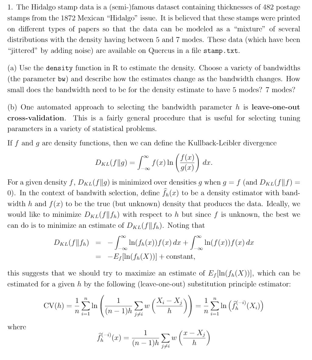
1. The Hidalgo stamp data is a (semi-)famous dataset containing thicknesses of 482 postage stamps from the 1872 Mexican "Hidalgo" issue. It is believed that these stamps were printed on different types of papers so that the data can be modeled as a "mixture" of several distributions with the density having between 5 and 7 modes. These data (which have been "jittered" by adding noise) are available on Quercus in a file stamp . txt. (a) Use the density function in R to estimate the density. Choose a variety of bandwidths (the parameter bw) and describe how the estimates change as the bandwidth changes. How small does the bandwidth need to be for the density estimate to have 5 modes? 7 modes? (b) One automated approach to selecting the bandwidth parameter h is leave-one-out cross-validation. This is a fairly general procedure that is useful for selecting tuning parameters in a variety of statistical problems. If f and g are density functions, then we can define the Kullback-Leibler divergence DKL(fig) = f(x) In f(2) d.x . For a given density f, DKL(fl|g) is minimized over densities g when g = f (and DKL(flIf) = 0). In the context of bandwith selection, define fr(x) to be a density estimator with band- width h and f(x) to be the truc (but unknown) density that produces the data. Ideally, we would like to minimize DKL(flIf) with respect to h but since f is unknown, the best we can do is to minimize an estimate of DKL(flIfh). Noting that DKL(filth) = - In(fr(x))f(x) dx + In(f(x))f(x) dx = -EflIn(fr (X))] + constant, this suggests that we should try to maximize an estimate of Ey[In(fr(X))], which can be estimated for a given h by the following (leave-one-out) substitution principle estimator: CV(h) = = Ew Xi Xj (n - 1)h = 1EIn (MK) (Xi)) ifi h where f -" ( x ) = 1 Xj (n - 1 )h ifi h