1.In a factorial design with two factors, if the effect of one factor appears to depend on the levels of the second factor, this is called

a.An interaction effect

b.A main effect

c.A factorial effect

d.An error

2.A study found that 50 pedestrians gave more money to a street beggar if the beggar had a cute and hungry-looking dog with them compared to if they were alone. The gender of the pedestrians was also noted. Which of the following sentences describes a simple effects analysis on these data?

a.The difference in donations when the beggar had a dog compared to not

b.The effect of having a dog compared to not on donations calculated separately for male and female pedestrians

c.The relative difference between male donations and female donations when the beggar had a dog compared to not

d.Using a graph to do one simple inspection of the mean donations from male and female pedestrians when the beggar had a dog or was alone

3.Simple effects analysis looks at:

a.The effect of one independent variable at individual levels of the dependent variable

b.The main effects of the independent variables, controlling for interaction effects

c.The effect of one independent variable at individual levels of the other independent variable

d.The difference between the main effects of two independent variables controlling for error

4.A study was conducted to look at whether caffeine improves productivity at work in different conditions. There were two independent variables. The first independent variable was email, which had two levels: 'email access' and 'no email access'. The second independent variable was caffeine, which also had two levels: 'caffeinated drink' and 'decaffeinated drink'.Different participants took part in each condition. Productivity was recorded at the end of the day on a scale of 0 (I may as well have stayed in bed) to 20 (wow! I got enough work done today to last all year). Looking at the group means in the table below, which of the following statements best describes the data?

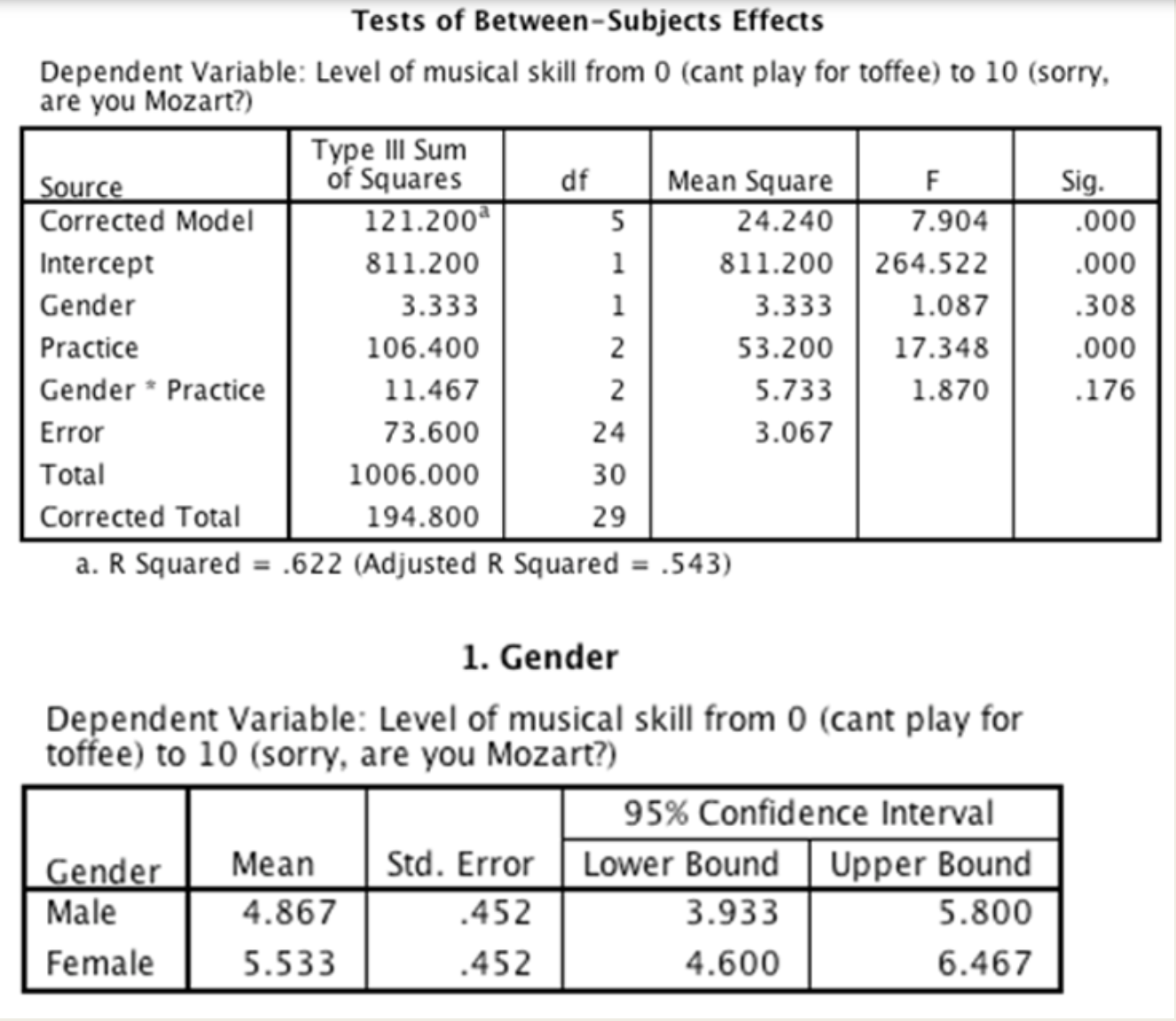
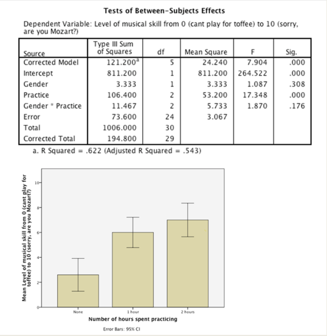
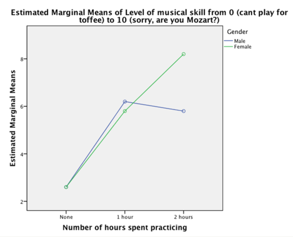
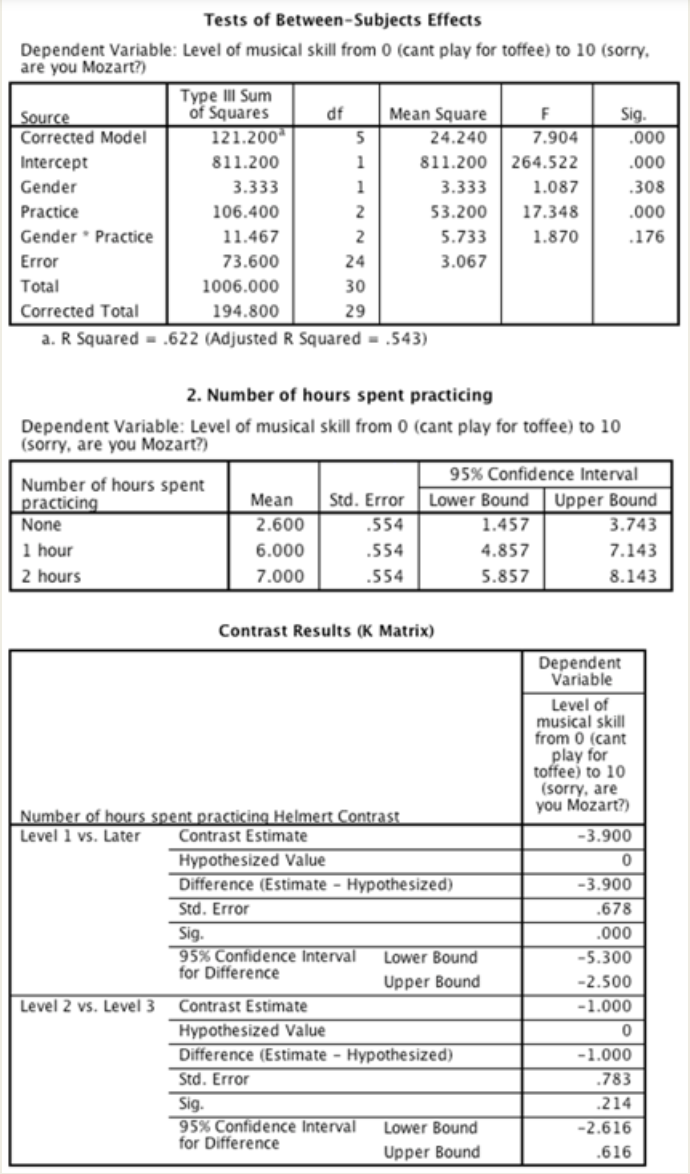
\f\fTests of Between-Subjects Effects Dependent Variable: Level of musical skill from 0 (cant play for toffee) to 10 (sorry, are you Mozart?) Type Ill Sum Source of Squares df Mean Square F Sig Corrected Model 121.200 24.240 7.904 000 Intercept 811.200 811.200 264.522 .000 Gender 3.333 3.333 1.087 .308 Practice 106.400 2 53.200 17.348 .000 Gender * Practice 11.467 2 5.733 1.870 .176 Error 73.600 24 3.067 Total 1006.000 30 Corrected Total 194.800 29 a. R Squared = .622 (Adjusted R Squared = .543) 1. Gender Dependent Variable: Level of musical skill from 0 (cant play for toffee) to 10 (sorry, are you Mozart?) 95% Confidence Interval Gender Mean Std. Error Lower Bound Upper Bound Male 4.867 .452 3.933 5.800 Female 5.533 .452 4.600 6.467Tests of Between-Subjects Effects Dependent Variable: Level of musical skill from 0 (cant play for toffee) to 10 (sorry, are you Mozart?) Type Ill Sum Source of Squares df Mean Square F Sig. Corrected Model 121.200 24.240 7.904 000 Intercept 811.200 811.200 264.522 .000 Gender 3.333 3.333 1.087 .308 Practice 106.400 2 53.200 17.348 .000 Gender * Practice 11.467 2 5.733 1.870 .176 Error 73.600 24 3.067 Total 1006.000 30 Corrected Total 194.800 29 a. R Squared = .622 (Adjusted R Squared = .543) Mean Level of musical skill from 0 (cant play for toffee) to 10 (sorry, are you Mozart?) None 1 hour 2 hours Number of hours spent practicing Error Bars: 95% CIEstimated Marginal Means of Level of musical skill from 0 (cant play for toffee) to 10 (sorry, are you Mozart?) Gender - Male Female Estimated Marginal Means None 1 hour 2 hours Number of hours spent practicingTests of Between-Subjects Effects Dependent Variable: Level of musical skill from 0 (cant play for toffee) to 10 (sorry. are you Mozart?) Type Ill Sum Source of Squares df Mean Square F Sig. Corrected Model 121.200 24.240 7.904 000 Intercept 811.200 811.200 264.522 .000 Gender 3.333 3.333 1.087 .308 Practice 106.400 2 53.200 17.348 000 Gender * Practice 11.467 5.733 1.870 .176 Error 73.600 24 3.067 Total 1006.000 30 Corrected Total 194.800 29 a. R Squared = .622 (Adjusted R Squared = .543) 2. Number of hours spent practicing Dependent Variable: Level of musical skill from 0 (cant play for toffee) to 10 (sorry, are you Mozart?) Number of hours spent 95% Confidence Interval practicing Mean Std. Error Lower Bound Upper Bound None 2.600 .554 1.457 3.743 1 hour 6.000 .554 4.857 7.143 2 hours 7.000 .554 5.857 8.143 Contrast Results (K Matrix) Dependent Variable Level of musical skill from 0 (cant play for toffee) to 10 (sorry, are Number of hours spent practicing Helmert Contrast you Mozart?) Level 1 vs. Later Contrast Estimate -3.900 Hypothesized Value 0 Difference (Estimate - Hypothesized) -3.900 Std. Error 678 Sig. 000 95% Confidence Interval for Difference Lower Bound -5.300 Upper Bound -2.500 Level 2 vs. Level 3 Contrast Estimate -1.000 Hypothesized Value 0 Difference (Estimate - Hypothesized) -1.000 Std. Error 783 Sig. .214 95% Confidence Interval Lower Bound for Difference -2.616 Upper Bound .616