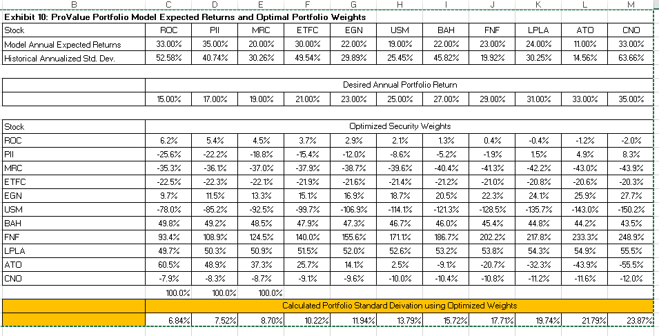
2. As is discussed in the case, the ProValue fund is likely to grow in the near future and because of that, Allison is considering making significant changes to the portfolio. In particular, she is considering adding two new stocks, ATO and CNO, to the nine that the fund is currently invested in. She is also interested in exploring the impact of introducing some short positions. Based on the portfolio optimization techniques that we discussed in class, prepare a short report highlighting the difference in performance that these changes are likely to make. Specifically, briefly analyze how the performance of the fund is likely to be affected: -- by using optimized portfolio weights rather than the current weights reported in Exhibit 8. -- by allowing short sales. -- by adding the two new stocks. Providing a few well-chosen graphs (for example, graphs comparing the efficient frontier before and after the changes) will help you make your points. You may also want to use some of the performance measures in Exhibit 4 (although this is not required). For both questions, you may need an estimate of the riskless interest rate. You can use a value of 0.25% per year (which is unusually low by long term historical standards, but reasonable for the period of the case). For question 2, you may want to use the analysis that we did in class (using Excel's solver) as a starting point. Note that your results may not exactly match those reported in Exhibit 10 of the case. This is not a problem. (I have checked and, for reasons that are a mystery to me, the results in Exhibit 10 are based on slightly different data than that provided with the case.) D Exhibit 10: ProValue Portfolio Model Expected Returns and Optimal Portfolio Weights Stock ROC PILI | MRC ETFC EGN Model Annual Expected Returns 33.00% 35.00% 20.00% 30.00% 22.00% Historical Annualized Std. Dev. 52.58% 40.74% 30.26% 49.54% 29.89% USMBAH 19.00% 22.00% 25.45% 45.82% FNFLPLA 23.00% 24.00% 19.92% 30.25% ATOCNO 11.00% 33.00% 14.56% 63.66% Desired Annual Portfolio Return 23.00% 25.00% 27.00% 15.00% 17.00% 19.00% 21.00% 29.00% 31.00% 33.00% 35.00% Stock ROC MRC ETFC EGN USM BAH ENE LPLA ATO CNO 6.2% -25.6% -35.3% -22.5% 9.7% -78.0% 49.8% 93.4% 49.7% 60.5% -7.9% 100.0% 5.4% -22.2% -36.1% -22.3% 11.5% -85.2% 49.2% 108.9% 50.3% 48.9% -8.3% 100.0% Optimized Security Weights 4.5% 3.7% 2.9% 2.1% 13% 0.4% -0.4% -18.8% -15.4% -12.0% -8.6% -5.2% -1.9% 1.5% -37.0% -37.9% -38.7% -39.6% -40.4% -41.3% -42.2% -22.1% -21.9% -21.6% -21.4% -21.2% -21.0% -20.8% 13.3% 15.1% 16.9% 18.7% 20.5% 22.3% 24.1% -92.5% -99.7% -106.9% - 114.1% -121.3% -128.5% -135.7% 48.5% 47.9% 47.3% 46.7% 46.0% 45.4% 44.8% 124.5% 140.0% 155.6% 171.1% 186.7% 202.2% 217.8% 50.9% 51.5% 52.0% 52.6% 53.2% 53.8% 54.3% 37.3% 25.7% 14.1% 2.5% -9.1% -20.7% -32.3% -8.7% -9.1% -9.6% -10.0% -10.4% -10.8% -11.2% 100.0% Calculated Portfolio Standard Deivation using Optimized Weights 8.70%. 10.227 . 11.94%| 13.79%. 15.72%4| 17.7174. 19.74% -1.2% 4.9% -43.0% -20.6% 25.9% -143.0% 44.2% 233.3% 54.9% -43.9% -11.6% -20% 8.3% -43.9% -20.3% 27.7% -150.2% 43.5% 248.9% 55.5% -55.5% - 12.0% 6.84% 7.52% 21.79%| 23.87% 2. As is discussed in the case, the ProValue fund is likely to grow in the near future and because of that, Allison is considering making significant changes to the portfolio. In particular, she is considering adding two new stocks, ATO and CNO, to the nine that the fund is currently invested in. She is also interested in exploring the impact of introducing some short positions. Based on the portfolio optimization techniques that we discussed in class, prepare a short report highlighting the difference in performance that these changes are likely to make. Specifically, briefly analyze how the performance of the fund is likely to be affected: -- by using optimized portfolio weights rather than the current weights reported in Exhibit 8. -- by allowing short sales. -- by adding the two new stocks. Providing a few well-chosen graphs (for example, graphs comparing the efficient frontier before and after the changes) will help you make your points. You may also want to use some of the performance measures in Exhibit 4 (although this is not required). For both questions, you may need an estimate of the riskless interest rate. You can use a value of 0.25% per year (which is unusually low by long term historical standards, but reasonable for the period of the case). For question 2, you may want to use the analysis that we did in class (using Excel's solver) as a starting point. Note that your results may not exactly match those reported in Exhibit 10 of the case. This is not a problem. (I have checked and, for reasons that are a mystery to me, the results in Exhibit 10 are based on slightly different data than that provided with the case.) D Exhibit 10: ProValue Portfolio Model Expected Returns and Optimal Portfolio Weights Stock ROC PILI | MRC ETFC EGN Model Annual Expected Returns 33.00% 35.00% 20.00% 30.00% 22.00% Historical Annualized Std. Dev. 52.58% 40.74% 30.26% 49.54% 29.89% USMBAH 19.00% 22.00% 25.45% 45.82% FNFLPLA 23.00% 24.00% 19.92% 30.25% ATOCNO 11.00% 33.00% 14.56% 63.66% Desired Annual Portfolio Return 23.00% 25.00% 27.00% 15.00% 17.00% 19.00% 21.00% 29.00% 31.00% 33.00% 35.00% Stock ROC MRC ETFC EGN USM BAH ENE LPLA ATO CNO 6.2% -25.6% -35.3% -22.5% 9.7% -78.0% 49.8% 93.4% 49.7% 60.5% -7.9% 100.0% 5.4% -22.2% -36.1% -22.3% 11.5% -85.2% 49.2% 108.9% 50.3% 48.9% -8.3% 100.0% Optimized Security Weights 4.5% 3.7% 2.9% 2.1% 13% 0.4% -0.4% -18.8% -15.4% -12.0% -8.6% -5.2% -1.9% 1.5% -37.0% -37.9% -38.7% -39.6% -40.4% -41.3% -42.2% -22.1% -21.9% -21.6% -21.4% -21.2% -21.0% -20.8% 13.3% 15.1% 16.9% 18.7% 20.5% 22.3% 24.1% -92.5% -99.7% -106.9% - 114.1% -121.3% -128.5% -135.7% 48.5% 47.9% 47.3% 46.7% 46.0% 45.4% 44.8% 124.5% 140.0% 155.6% 171.1% 186.7% 202.2% 217.8% 50.9% 51.5% 52.0% 52.6% 53.2% 53.8% 54.3% 37.3% 25.7% 14.1% 2.5% -9.1% -20.7% -32.3% -8.7% -9.1% -9.6% -10.0% -10.4% -10.8% -11.2% 100.0% Calculated Portfolio Standard Deivation using Optimized Weights 8.70%. 10.227 . 11.94%| 13.79%. 15.72%4| 17.7174. 19.74% -1.2% 4.9% -43.0% -20.6% 25.9% -143.0% 44.2% 233.3% 54.9% -43.9% -11.6% -20% 8.3% -43.9% -20.3% 27.7% -150.2% 43.5% 248.9% 55.5% -55.5% - 12.0% 6.84% 7.52% 21.79%| 23.87%