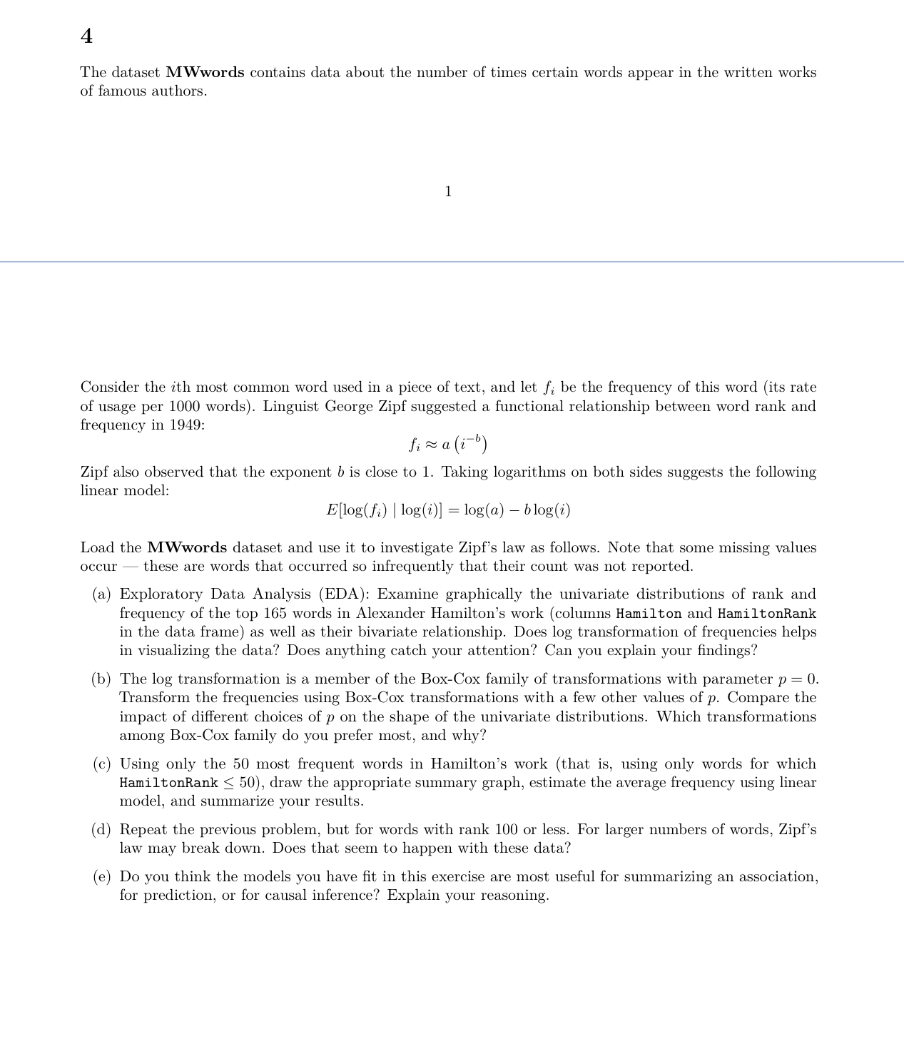
4 The dataset MWwords contains data about the number of times certain words appear in the written works of famous authors. Consider the ith most common word used in a piece of text, and let f,- be the frequency of this word (its rate of usage per 1000 words). Linguist George Zipf suggested a functional relationship between word rank and frequency in 1949: f, w a. (15-?) Zipf also observed that the exponent b is close to 1. Taking logarithms on both sides suggests the following linear model: 1300300 | 10%)] :1Os(a) 51030) Load the MWwords dataset and use it to investigate Zipf's law as follows. Note that some missing values occur these are words that occurred so infrequently that their count was not reported. (a) Exploratory Data Analysis (EDA): Examine graphically the unjvariate distributions of rank and frequency of the top 165 words in Alexander Hamilton's work (columns Hamilton and HamiltonRank in the data frame) as well as their bivariate relationship. Does log transformation of frequencies helps in visualizing the data? Does anything catch your attention? Can you explain your ndings? (b) The log transformation is a member of the Box-Cox family of transformations with parameter p = 0. Transform the frequencies using Box-Cox transformations with a few other values of p. Compare the impact of different choices of p on the shape of the univariate distributions. Which transformations among Box-Cox family do you prefer most, and why? (c) Using only the 50 most frequent words in Hamilton's work (that is, using only words for which Hami 1t onRank S 50), draw the appropriate summary graph, estimate the average frequency using linear model, and summarize your results. (d) Repeat the previous problem, but for words with rank 100 or less. For larger numbers of words, Zipf's law may break down. Does that seem to happen with these data? (e) Do you think the models you have t in this exercise are most useful for summarizing an association, for prediction, or for causal inference? Explain your reasoning