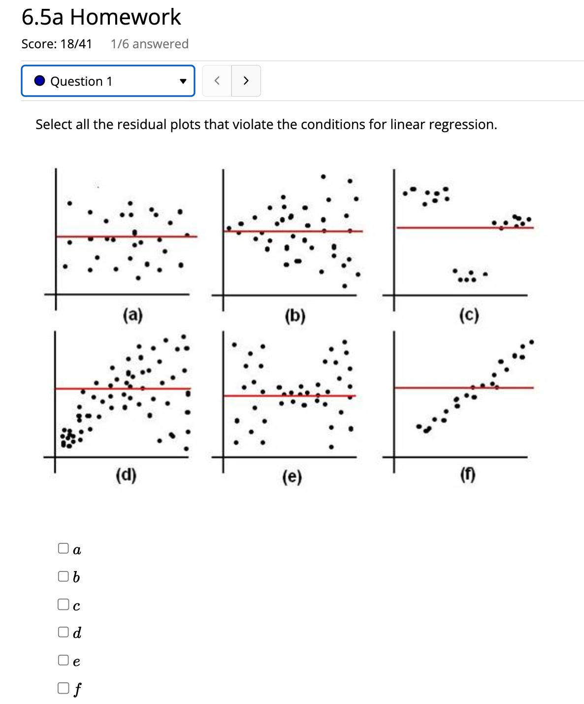
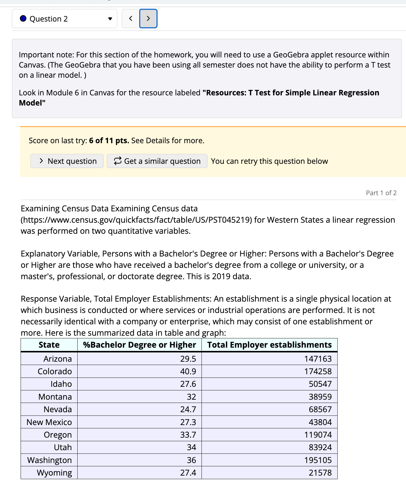
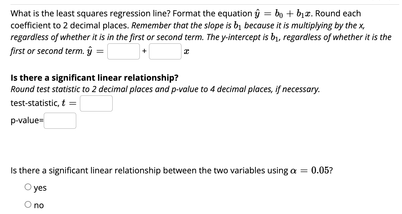
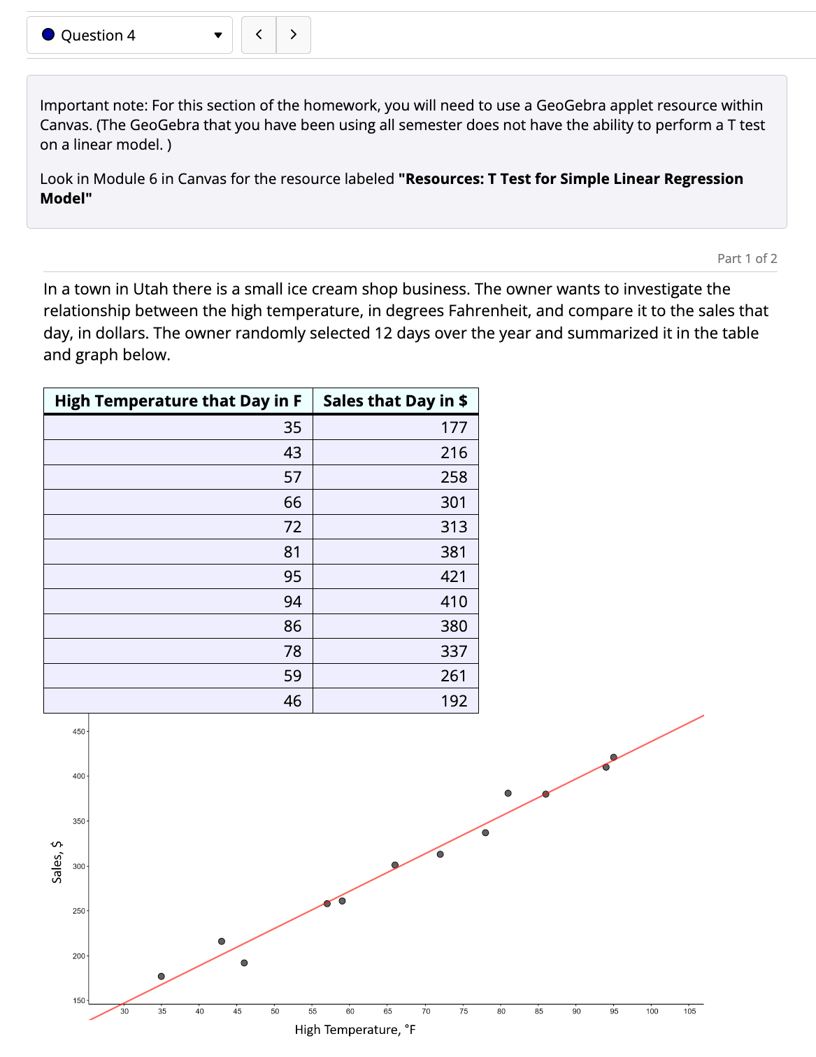
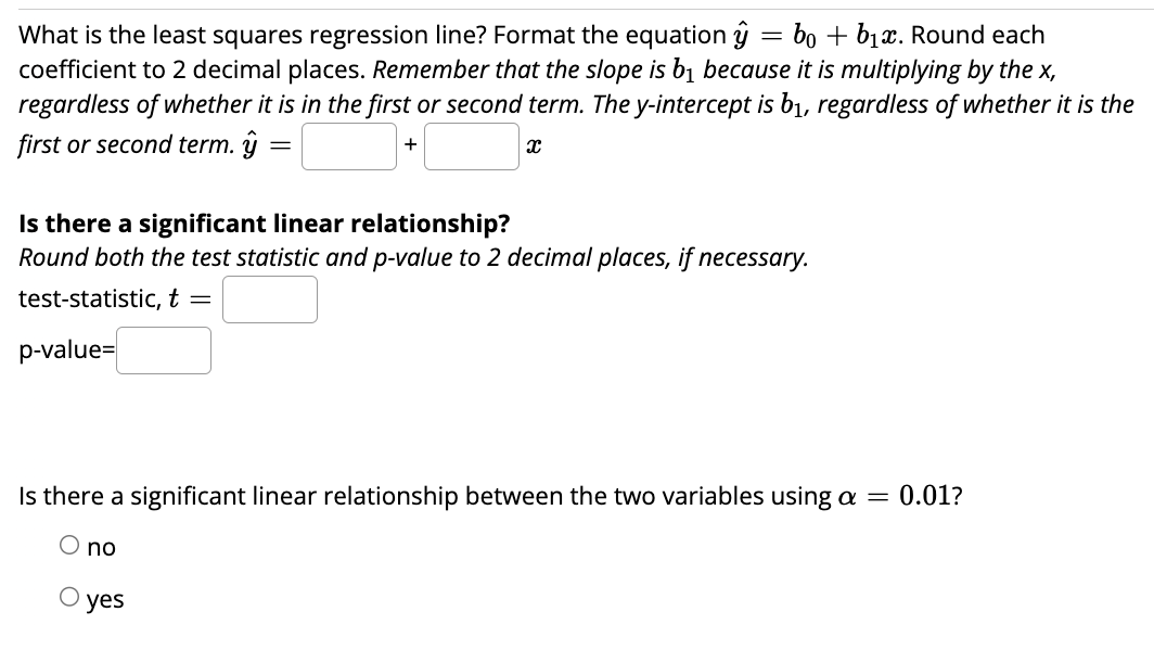
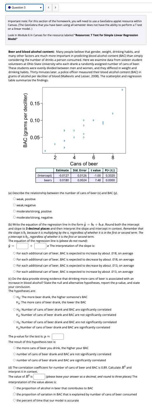
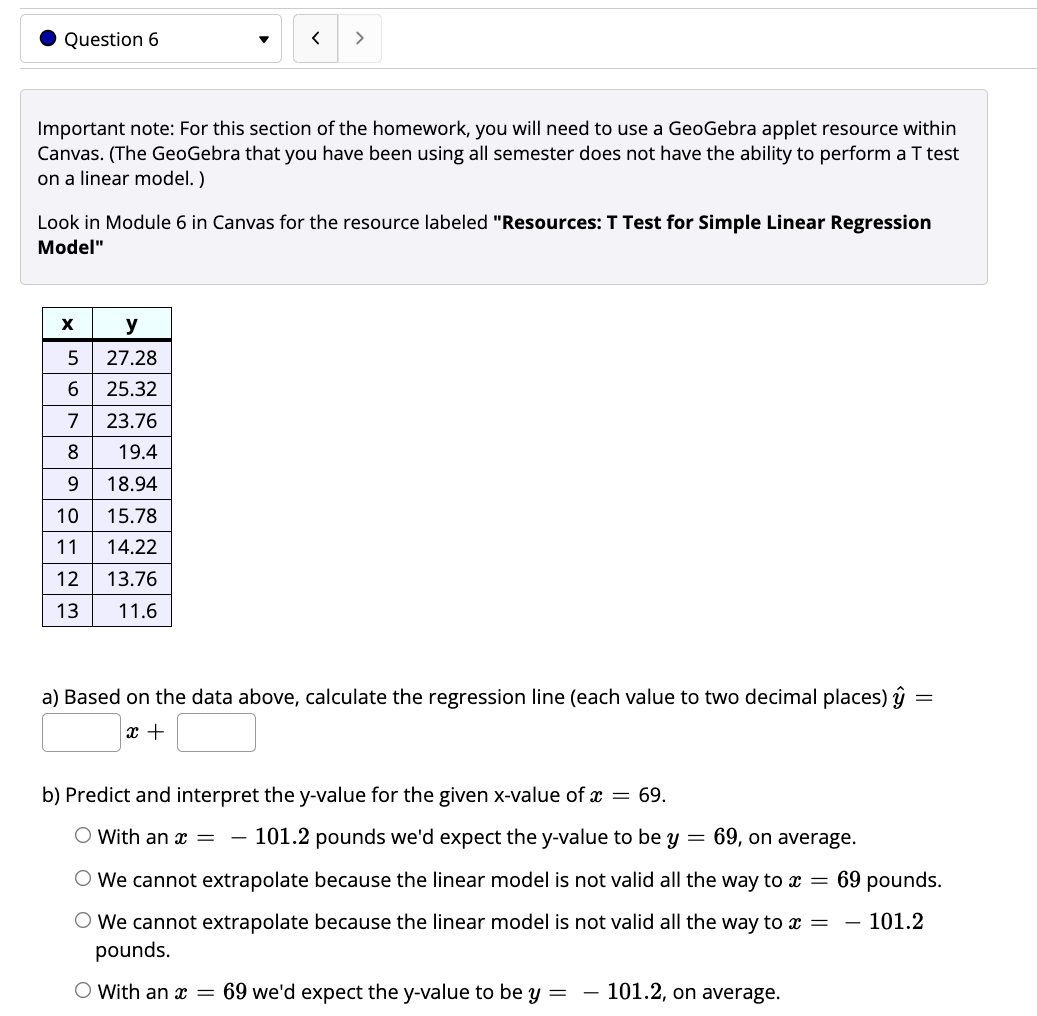
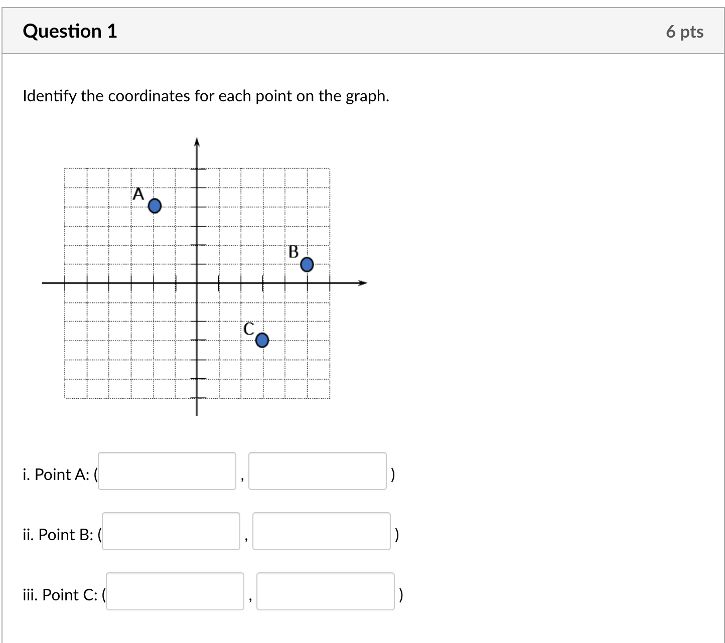
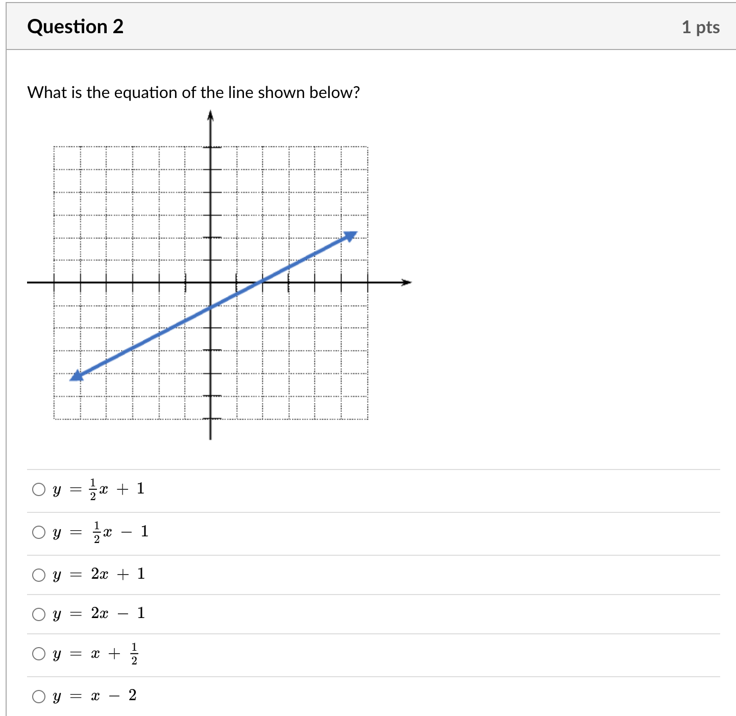
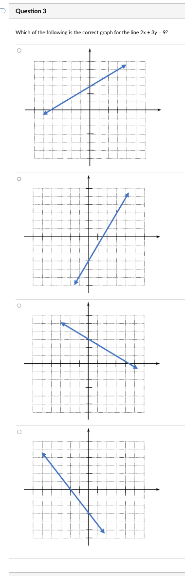
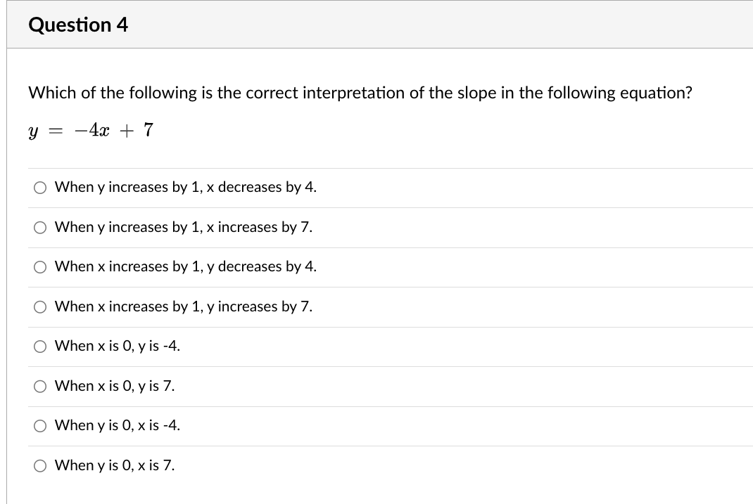
6.5a Homework Score: 18,141 1/6 answered 0 Question 1 v Select all the residual plots that violate the conditions for linear regression. 0' o o o... .. .0. .0 0: . o .. o. o I C . .... . . o .n a: o ...o I .00. . O ..' . .. 3" . . I o .. ." .139: , ' " (d) (e) (f) oer-g: l'l ma. ""h 0 Question 2 v Next question 8 Get a similar question You can retry this question below Part1 of2 Examining Census Data Examining Census data (https://www.census.govlquickfacts/fact/table/US/PST045219) for Western States a linear regression was performed on two quantitative variables. Explanatory Variable, Persons with a Bachelor's Degree or Higher: Persons with a Bachelor's Degree or Higher are those who have received a bachelor's degree from a college or university, or a master's, professional, or doctorate degree. This is 2019 data. Response Variable, Total Employer Establishments: An establishment is a single physical location at which business is conducted or where services or industrial operations are performed. It is not necessarily identical with a company or enterprise, which may consist of one establishment or more. Here is the summarized data in table and graph: State %Bachelor Degree or Higher Total Employer establishments Arizona 29.5 147163 Colorado 40.9 174258 Idaho 27.6 50547 Montana 32 38959 Nevada 24.7 68567 New Mexico 27.3 43804 Oregon 33.7 119074 Utah 34 83924 Washington 36 195105 Wyoming 27.4 21578 What is the least squares regression line? Format the equation Q : bu + b133, Round each coefficient to 2 decimal places. Remember that the slope is b1 because it is multiplying by the X, regardless of whether it is in the first or second term. The yintercept is 131, regardless of whether it is the first or second term. 3} : + :13 Is there a significant linear relationship? Round test statistic to 2 decimal places and p-value to 4 decimal places, if necessary. test-statistic, t : p-value= Is there a significant linear relationship between the two variables using or : 0.05? 0 yes 0 no 0 Question 4 v Important note: For this section of the homework, you will need to use a GeoGebra applet resource within Canvas. (The GeoGebra that you have been using all semester does not have the ability to perform a T test on a linear model.) Look in Module 6 in Canvas for the resource labeled "Resources: T Test for Simple Linear Regression Model" Part1 of2 In a town in Utah there is a small ice cream shop business. The owner wants to investigate the relationship between the high temperature, in degrees Fahrenheit, and compare it to the sales that day, in dollars. The owner randomly selected 12 days over the year and summarized it in the table and graph below. High Temperature that Day in F Sales that Day in S 35 177 43 216 57 258 66 301 72 313 81 381 95 421 94 410 86 380 78 337 59 261 46 192 400 350 300 Sales, 3 250 200 150 ED 35 4E] .15 50 55 t] 65 7E] 75 RC- 85 9E] 95 1 1 [15 High Temperature, DF What is the least squares regression line? Format the equation y = bo + bix. Round each coefficient to 2 decimal places. Remember that the slope is b1 because it is multiplying by the x, regardless of whether it is in the first or second term. The y-intercept is b1, regardless of whether it is the first or second term. y Is there a significant linear relationship? Round both the test statistic and p-value to 2 decimal places, if necessary. test-statistic, t = p-value= Is there a significant linear relationship between the two variables using a = 0.01? O no O yes. Question 5 Important note: For this section of the homework, you will need to use a GeoGebra applet resource within Canvas. (The GeoGebra that you have been using all semester does not have the ability to perform a T test on a linear model. ) Look in Module 6 in Canvas for the resource labeled "Resources: T Test for Simple Linear Regression Model" Beer and blood alcohol content: Many people believe that gender, weight, drinking habits, and many other factors are much more important in predicting blood alcohol content (BAC) than simply considering the number of drinks a person consumed. Here we examine data from sixteen student volunteers at Ohio State University who each drank a randomly assigned number of cans of beer. These students were evenly divided between men and women, and they differed in weight and drinking habits. Thirty minutes later, a police officer measured their blood alcohol content (BAC) in grams of alcohol per deciliter of blood (Malkevitcand Lesser, 2008). The scatterplot and regression table summarize the findings. 0.15 BAC (grams per deciliter) 0.10 0.05 2 4 6 8 Cans of beer Estimate Std. Error t value P(>[t[) (Intercept) 0.0127 0.0126 -1.00 0.3320 beers 0.0180 0.0024 7.48 0.0000 (a) Describe the relationship between the number of cans of beer (x) and BAC (y). O weak, positive O weak,negative moderate/strong, positive moderate/strong, negative (b) Write the equation of the regression line in the form y = bo + bit. Round both the intercept and slope to 3 decimal places and then interpret the slope and intercept in context. Remember that the slope is by because it is multiplying by the x, regardless of whether it is in the first or second term. The y-intercept is by, regardless of whether it is the first or second term. The equation of the regression line is (please do not round): y = + The interpretation of the slope is: O For each additional can of beer, BAC is expected to increase by about .018, on average O For each additional can of beer, BAC is expected to decrease by about .018, on average O For each additional can of beer, BAC is expected to decrease by about .013, on average O For each additional can of beer, BAC is expected to increase by about .013, on average (c) Do the data provide strong evidence that drinking more cans of beer is associated with an increase in blood alcohol? State the null and alternative hypotheses, report the p-value, and state your conclusion. The hypotheses are: Ho: The more beer drank, the higher someone's BAC Ha: The more cans of beer drank, the lower the BAC O Ho: Number of cans of beer drank and BAC are significantly correlated Ha: Number of cans of beer drank and BAC are not significantly correlated O Ho: Number of cans of beer drank and BAC are not significantly correlated Ha:Number of cans of beer drank and BAC are significantly correlated The p-value for the test is: p The result of this hypothesis test is: O the more cans of beer you drink, the higher your BAC O number of cans of beer drank and BAC are not significantly correlated O number of cans of beer drank and BAC are significantly correlated (d) The correlation coefficient for number of cans of beer and BAC is 0.89. Calculate R" and interpret it in context. The value of R is (please leave your answer as a decimal, and round to three places) The interpretation of the value above is: the proportion of alcohol in beer that contributes to BAC the proportion of variation in BAC that is explained by number of cans of beer consumed the percent of time that our model is accurate. Question 6 v ( > Important note: For this section of the homework. you will need to use a GeoGebra applet resource within Canvas. (The GeoGebra that you have been using all semester does not have the ability to perform a T test on a linear model.) Look in Module 6 in Canvas for the resource labeled "Resources: T Test for Simple Linear Regression Model" x y 5 27.28 6 25.32 7 23.76 8 19.4 9 18.94 10 15.78 11 14.22 12 13.76 13 11.6 a) Based on the data above, calculate the regression line (each value to two decimal places) 3} = a: + b) Predict and interpret the yvalue for the given xvalue of a: = 69. 0 With an a: : 101.2 pounds we'd expect the y-value to be y : 69. on average. 0 We cannot extrapolate because the linear model is not valid all the way to a: = 69 pounds. 0 We cannot extrapolate because the linear model is not valid all the way to :1: : 101.2 pounds. 0 With an a: : 69 we'd expect the yvalue to be 3; : 101.2, on average. Question 1 6 pts Identify the coordinates for each point on the graph. i. Point A: ( , ) ii. Point B: ( , ) iii. Point C: ( , ) Question 2 1 pts What is the equation of the line shown below? -..... ..L... ... .... Oy = a+1 Oy = ta - 1 Oy = 2x + 1 Oy = 2x - 1 Oy = atz Oy = x - 2Question 3 Which of the following is the correct graph for the line 2x + 3y = 9? O O OQuestion 4 Which of the following is the correct interpretation of the slope in the following equation? y = -4x + 7 O When y increases by 1, x decreases by 4. O When y increases by 1, x increases by 7. O When x increases by 1, y decreases by 4. O When x increases by 1, y increases by 7. O When x is O, y is -4. O When x is O, y is 7. O When y is O, x is -4. O When y is 0, x is 7