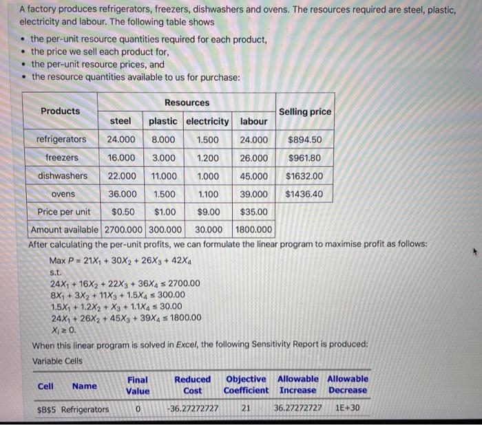
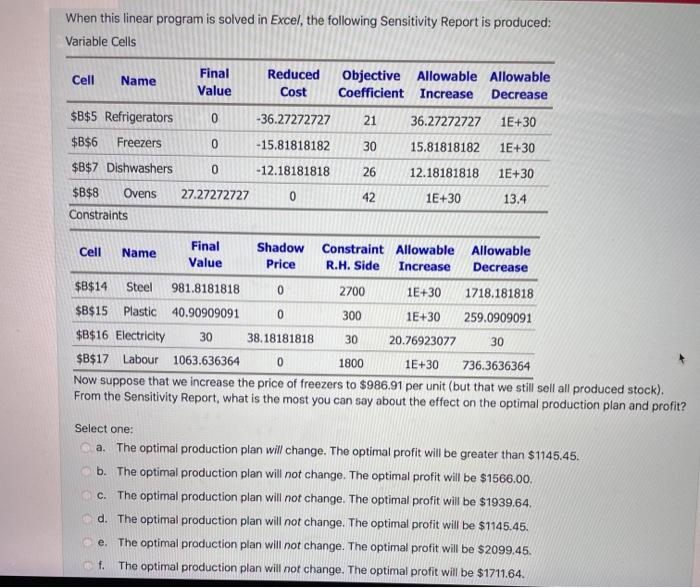
A factory produces refrigerators, freezers, dishwashers and ovens. The resources required are steel, plastic, electricity and labour. The following table shows the per-unit resource quantities required for each product, the price we sell each product for, the per-unit resource prices, and the resource quantities available to us for purchase: Resources Products Selling price steel plastic electricity labour refrigerators 24.000 8.000 1.500 24.000 $894.50 freezers 16.000 3.000 1.200 26.000 $961.80 dishwashers 22.000 11.000 1.000 45.000 $1632.00 ovens 36.000 1.500 1.100 39.000 $1436.40 Price per unit $0.50 $1.00 $9.00 $35.00 Amount available 2700.000 300.000 30.000 1800.000 After calculating the per-unit profits, we can formulate the linear program to maximise profit as follows: Max P = 21X1 + 30X2 + 26X3 + 42X4 s.t. 24X1 + 16X2 + 22X3 + 36X4 s 2700.00 8X1 + 3X2 + 11X3 +1.5X4 s 300.00 1.5X1 +1.2X2 + X3 + 1.1X4 s 30.00 24X1 + 26X2 + 45X3 + 39X4 S 1800.00 X/20. When this linear program is solved in Excel, the following Sensitivity Report is produced: Variable Cells Final Reduced Objective Allowable Allowable Cell Name Value Cost Coefficient Increase Decrease $B$5 Refrigerators 0 -36.27272727 21 36.27272727 1E+30 When this linear program is solved in Excel, the following Sensitivity Report is produced: Variable Cells Cell Name Final Value Reduced Cost Objective Allowable Allowable Coefficient Increase Decrease 0 -36.27272727 21 1E+30 0 -15.81818182 30 $B$5 Refrigerators $B$6 Freezers $B$7 Dishwashers $B$8 Ovens 1E+30 36.27272727 15.81818182 12.18181818 1E+30 0 -12.18181818 26 1E+30 27.27272727 0 42 13.4 Constraints Final Shadow Cell Constraint Allowable Name Allowable Value Price R.H. Side Increase Decrease $B$14 Steel 981.8181818 0 2700 1E+30 1718.181818 $B$15 Plastic 40.90909091 0 300 1E+30 259.0909091 $B$16 Electricity 30 38.18181818 30 20.76923077 30 $B$17 Labour 1063.636364 0 1800 1E+30 736.3636364 Now suppose that we increase the price of freezers to $986.91 per unit (but that we still sell all produced stock). From the Sensitivity Report, what is the most you can say about the effect on the optimal production plan and profit? Select one: a. The optimal production plan will change. The optimal profit will be greater than $1145.45. b. The optimal production plan will not change. The optimal profit will be $1566.00, c. The optimal production plan will not change. The optimal profit will be $1939.64. d. The optimal production plan will not change. The optimal profit will be $1145.45. e. The optimal production plan will not change. The optimal profit will be $2099.45 f. The optimal production plan will not change. The optimal profit will be $1711.64. A factory produces refrigerators, freezers, dishwashers and ovens. The resources required are steel, plastic, electricity and labour. The following table shows the per-unit resource quantities required for each product, the price we sell each product for, the per-unit resource prices, and the resource quantities available to us for purchase: Resources Products Selling price steel plastic electricity labour refrigerators 24.000 8.000 1.500 24.000 $894.50 freezers 16.000 3.000 1.200 26.000 $961.80 dishwashers 22.000 11.000 1.000 45.000 $1632.00 ovens 36.000 1.500 1.100 39.000 $1436.40 Price per unit $0.50 $1.00 $9.00 $35.00 Amount available 2700.000 300.000 30.000 1800.000 After calculating the per-unit profits, we can formulate the linear program to maximise profit as follows: Max P = 21X1 + 30X2 + 26X3 + 42X4 s.t. 24X1 + 16X2 + 22X3 + 36X4 s 2700.00 8X1 + 3X2 + 11X3 +1.5X4 s 300.00 1.5X1 +1.2X2 + X3 + 1.1X4 s 30.00 24X1 + 26X2 + 45X3 + 39X4 S 1800.00 X/20. When this linear program is solved in Excel, the following Sensitivity Report is produced: Variable Cells Final Reduced Objective Allowable Allowable Cell Name Value Cost Coefficient Increase Decrease $B$5 Refrigerators 0 -36.27272727 21 36.27272727 1E+30 When this linear program is solved in Excel, the following Sensitivity Report is produced: Variable Cells Cell Name Final Value Reduced Cost Objective Allowable Allowable Coefficient Increase Decrease 0 -36.27272727 21 1E+30 0 -15.81818182 30 $B$5 Refrigerators $B$6 Freezers $B$7 Dishwashers $B$8 Ovens 1E+30 36.27272727 15.81818182 12.18181818 1E+30 0 -12.18181818 26 1E+30 27.27272727 0 42 13.4 Constraints Final Shadow Cell Constraint Allowable Name Allowable Value Price R.H. Side Increase Decrease $B$14 Steel 981.8181818 0 2700 1E+30 1718.181818 $B$15 Plastic 40.90909091 0 300 1E+30 259.0909091 $B$16 Electricity 30 38.18181818 30 20.76923077 30 $B$17 Labour 1063.636364 0 1800 1E+30 736.3636364 Now suppose that we increase the price of freezers to $986.91 per unit (but that we still sell all produced stock). From the Sensitivity Report, what is the most you can say about the effect on the optimal production plan and profit? Select one: a. The optimal production plan will change. The optimal profit will be greater than $1145.45. b. The optimal production plan will not change. The optimal profit will be $1566.00, c. The optimal production plan will not change. The optimal profit will be $1939.64. d. The optimal production plan will not change. The optimal profit will be $1145.45. e. The optimal production plan will not change. The optimal profit will be $2099.45 f. The optimal production plan will not change. The optimal profit will be $1711.64